Extracting the Centerline and Track Boundary from a Map Image
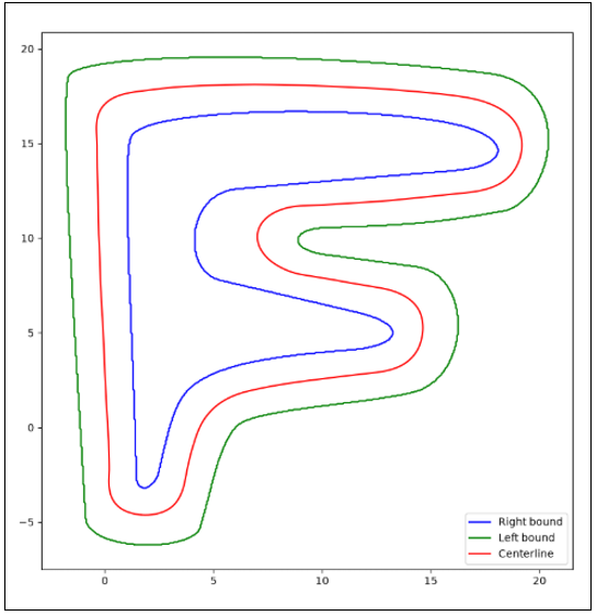
This stage extracts the track’s Centerline and Wall boundary from the occupancy grid map (/map) obtained with SLAM. It is the front part of global_planner_node in the gb_optimizer package — the first step of the Global Planning pipeline, producing the input for Global Trajectory Optimization: IQP/SP.
Three things are extracted — ① Centerline (closed loop through the middle of the track, the reference for the $s$ coordinate) ② Track width (distance to the left/right wall at each point) ③ Wall boundary (the actual walls — used for safety checks and avoidance clamping)
Pipeline Diagram
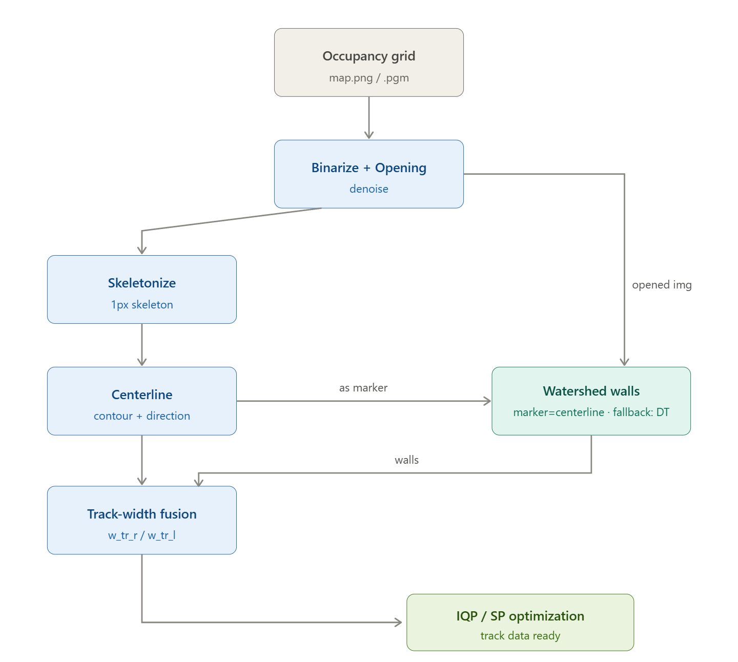
The information is refined in the order occupancy grid → 1-px skeleton → metric coordinates + width. The binary image splits into two branches — the skeleton (Centerline) and the watershed boundary — which meet again at the width computation. The computed widths are then used as the input to the alpha box constraints when optimizing the IQP & SP lines.
Step-by-Step Explanation
1. Map Loading + Binarization
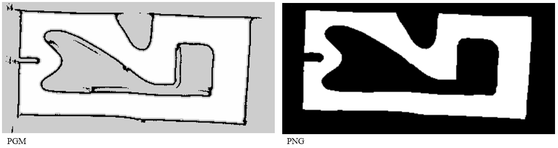 Step 1 — map loading / binarization
The node reads the occupancy grid published by map_server (or a saved map.png). Pixels whose occupancy value is below occupancy_grid_threshold (free space) are binarized to white (255).
The map loaded by map_server consists of an image ([map name].pgm or [map name].png) and a metadata yaml ([map name].yaml). This yaml holds the resolution and origin used to interpret pixels as real-world coordinates, and it is used for the pixel→meter conversion in step 3.
1
2
3
4
5
6
7
# stack_master/maps/[map name]/[map name].yaml
image: [map name].pgm
resolution: 0.05          # m/pixel — real size of one pixel
origin: [-8.21, -12.4, 0] # real coordinates of the map's bottom-left pixel [x, y, yaw]
occupied_thresh: 0.65     # occupied (wall) above this value
free_thresh: 0.196        # free space below this value
negate: 0                 # whether black/white are inverted
resolution and origin are the $r$ and $(o_x, o_y)$ of the conversion formula below ($x_m = \text{col}\cdot r + o_x$). In other words, this yaml file is what converts the map’s pixel coordinates into real metric coordinates.
2. Skeletonization
The filled driving area is thinned down to a 1-px centerline, extracting an unbroken skeleton from the closed loop.
3. Centerline Extraction
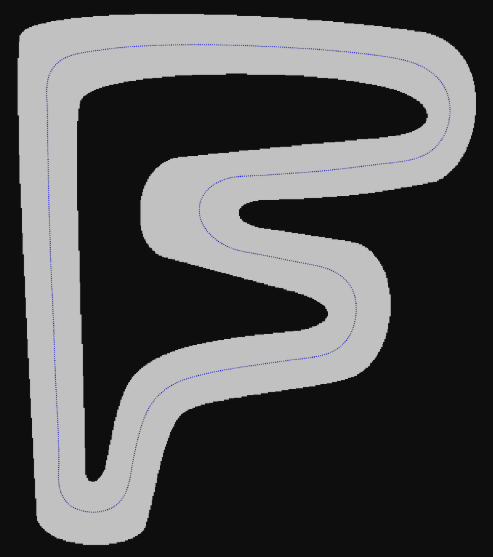
Closed curves (contours) are found in the skeleton image, and the closed loop corresponding to the track loop is taken as the centerline. If there are multiple candidate loops, the shortest one is selected to capture the inner loop. The selected centerline is still in pixel coordinates, so it is converted to real metric coordinates using the resolution and origin read from the yaml earlier.
Here $r$ is resolution and $(o_x, o_y)$ is origin.
4. Direction Alignment (CCW/CW)
The extracted centerline has a direction given by the order of its points, and this direction may be opposite to the vehicle’s actual driving direction. The node therefore compares the vehicle’s initial heading with the centerline’s direction and, if they disagree, reverses the point order to match. This aligns the direction of the driving coordinate ($s$) with the actual driving direction; if the reverse_mapping option is enabled, the direction is flipped once more here.
5. Wall Boundary Extraction: Watershed

The watershed algorithm separates the track’s left and right walls. Two concepts are used here.
- Distance transform: an image of the same size as the original map, where each pixel of the driving area (white) is replaced with the distance to the nearest wall. Pixels next to a wall are close to 0 and values grow toward the middle of the track width, so it becomes an image whose brightness shows how far each point is from the walls.
- Watershed: an algorithm that grows different seed regions starting from the lowest values, and splits the space along the ridge where two neighboring regions meet.
The sign of the distance transform is flipped so that values get smaller toward the track center, far from the walls. With the centerline set as the seed region, applying watershed expands the left and right regions from the centerline, and the boundary where the two regions meet is detected as the left/right walls.
6. Track Width Fusion + Centerline Publishing
Each point of the extracted centerline is annotated with the distances to the left/right walls found in the previous step as its width information. Curvature ($\kappa$) and heading ($\psi$) are computed separately from the width, by treating the centerline as a smooth curve (spline) and numerically differentiating it, and are recorded at each point as well.
| Data | Source | Purpose |
|---|---|---|
d_left, d_right | watershed boundary | alpha box constraints for IQP/SP |
| boundary (left/right walls) | watershed | safety checks and avoidance clamping (actual walls) |
psi, kappa | Centerline spline | curvature / heading |
The resulting Centerline and Wall boundary values are saved to global_waypoints.json.
Inputs and Outputs
Parameters come in through two paths. The values themselves come from stack_master/config/global_planner_params.yaml, while the switches that change per run (map, direction, simulation or not, etc.) are passed as arguments of raceline_generator.launch.xml.
Values from config (global_planner_params.yaml)
| Parameter | Value | Description |
|---|---|---|
occupancy_grid_threshold | 10 | Threshold for classifying occupancy grid free space (node default is 50, but 10 is used in the config) |
required_laps | 1 | Number of laps to drive before optimization in driving mode |
Values passed as launch arguments (raceline_generator.launch.xml)
| Argument | Parameter it feeds | Description |
|---|---|---|
map | map / map_dir | Map name to use (subfolder of stack_master/maps/) |
sim | racecar_version | true selects the SIM config folder, false the CAR one |
reverse | reverse_mapping | Reverses the raceline direction |
show_plots | show_plots | Shows extraction/optimization debug plots |
Published topics: /centerline_waypoints (+/markers), /trackbounds/markers. The Centerline (blue spheres) and Wall boundary can be checked in RViz.
Running It Directly in the UNICORN Racing Stack
This stack is based on the UNICORN Racing Stack. ROS 2 Jazzy runs in a single conda environment without a system ROS installation. Enter the environment with the
unicornalias.
1. Enter the Environment + Build
1
2
unicorn          # enter the conda environment
cbuild           # build
If it is already built, you can skip this.
2. Run the raceline_generator Launch File
The centerline and wall boundary extraction stage does not run as a standalone node — it runs as part of global_planner_node. Run everything at once through raceline_generator.launch.xml.
1
2
3
4
# Generate the raceline from a saved map (includes Centerline / Wall boundary extraction)
ros2 launch stack_master raceline_generator.launch.xml map:=f sim:=true
# map:=map name
# On the real car use sim:=false (CAR config) / reverse direction with reverse:=true / show result plots with show_plots:=true
Checking the result: subscribe to
/centerline_waypoints/markers(blue spheres) and/trackbounds/markers(green/yellow) in RViz. Debug plots can be shown withshow_plots:=true.
Execution Results
These are the outputs of running raceline_generator.launch.xml map:=f sim:=true.
1) Execution log — the process of loading the map and extracting the Centerline and wall boundary is printed to the log.
1
2
3
4
5
6
[map_io]: Read map .../maps/f/f.png: 545 X 322 map @ 0.05 m/cell
[global_planner]: resolved source map dir -> .../maps/f
[global_planner_node] (1680, 2)
[global_planner_node] Direction of the centerline ...
[global_planner]: Using watershed for track bound extraction...
[global_planner]: Start Global Trajectory optimization with iterative minimum curvature...
The log confirms that the extracted Centerline has 1680 points and that the track boundary was extracted with watershed.
2) Debug visualization (show_plots:=true) — plots printed directly by the node while running, used to visually confirm the extraction completed correctly. ① Binary map + skeleton ② Metric-coordinate Centerline + Left/Right boundary (red = Centerline, blue = Right boundary, green = Left boundary) ③ Direction alignment check (first two points):
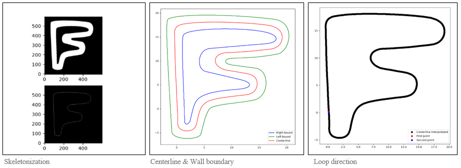
In the middle figure, everything is fine if the Centerline (red) passes right through the middle of the left/right walls. If the direction of the first two points (red→blue) in the right figure is opposite to what you intend, flip it with reverse:=true.
3) RViz check — the Centerline markers appear on top of the occupancy grid map (/map) served by map_server. The blue line (Centerline) follows the middle of the white driving area (the F-shaped track):
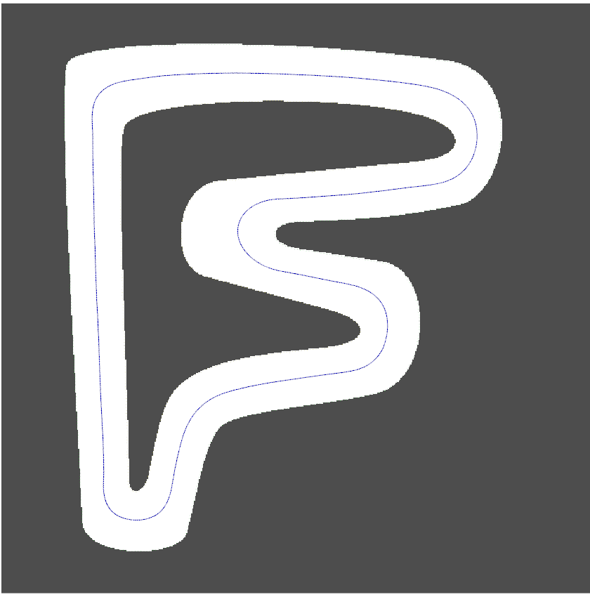 RViz: occupancy grid map + centerline markers
The marker topics are published with default QoS (the node stays alive spinning), so if you keep RViz open while the node is up, /centerline_waypoints/markers and /trackbounds/markers update in real time. (For reference, only /map is subscribed with TRANSIENT_LOCAL to match map_server’s latched setting.)
4) Artifacts — all extraction/optimization results are saved in stack_master/maps/f/. The Centerline and Wall boundary are stored together in global_waypoints.json.
The figures and logs above are the actual outputs of running map
f(the F-shaped track) in the UNICORN Racing Stack.
Wrap-up
This post covered the process of extracting the Centerline, Track width, and Wall boundary from a SLAM occupancy grid map. The track data, refined through map binarization → skeletonization → centerline extraction and direction alignment → watershed wall separation → width fusion, is saved to global_waypoints.json and becomes the foundation of the Global Planning pipeline.