Lane Change Planner: Overtaking Dynamic Obstacles with Lanes

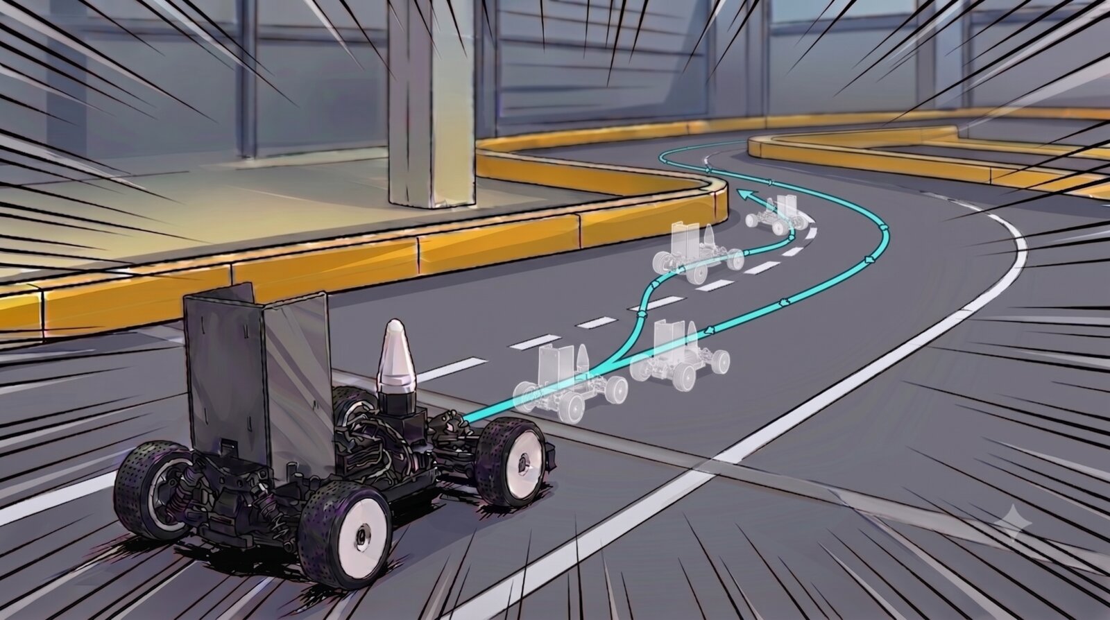
Dynamic obstacle avoidance is essential for successful overtaking — but pulling off an overtake on a narrow track, using your own state, the opponent’s state, and the track information together, is a genuinely hard problem.

Approaches like MPC that plan per-step actions over both cars’ timesteps, or that compute avoidance trajectories with a constrained solver, produce solutions that are hard to predict and cannot guarantee a feasible answer at every moment. They are tricky to use as-is in the RoboRacer domain, where variables arise constantly.

Considering these limits, the UNICORN Racing team handles narrow tracks with a simple dynamic avoidance algorithm that leverages pre-built lane information.

This post covers the Lane Change Planner: two lanes are built in advance to the left and right of the optimal line, and when an opponent blocks the way, the planner generates — in real time — an avoidance path that merges onto the free lane and then returns to the optimal line.

How It Works

Related code: planner/lane_change_planner/lane_change_planner/change_avoidance_node.py

The node builds the left/right lanes once at startup, then repeats the flow below every frame. Each step’s parameters can be adjusted live with rqt while driving.

1. Lane selection: picks the free lane, left or right, from the obstacle and track information.
2. d-profile generation: plans the lateral-displacement $d$ profile that moves onto that lane and then peels back to the optimal line.
3. Smoothing/validation: converts it to an $(x, y)$ curve, smooths it, and publishes it if the path stays inside the track.

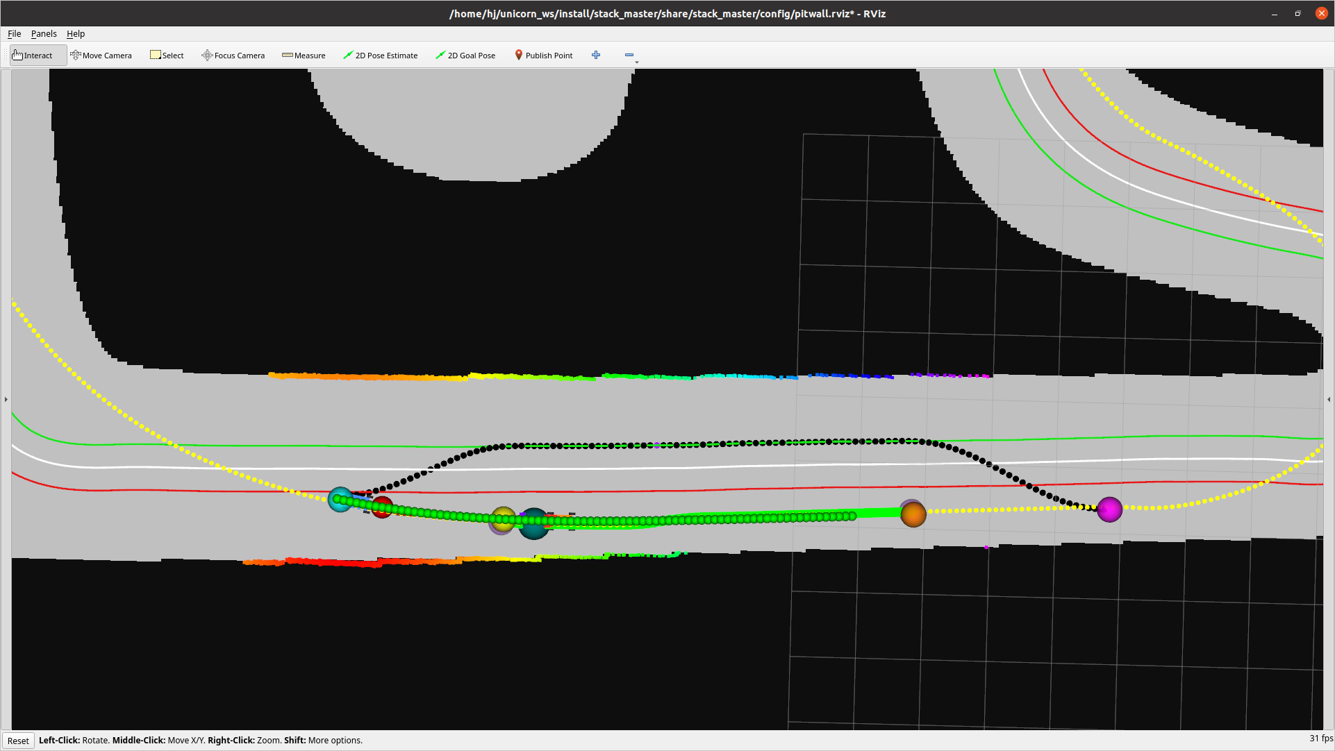
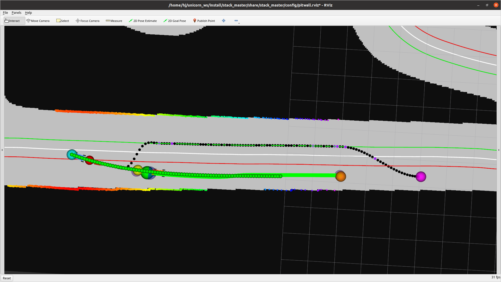
White = centerline, green/red = the pre-built left/right lanes, yellow dashed = the learned trajectory of the car ahead, black dashed = the generated avoidance path.

The black dashed line (the avoidance path) smoothly joins the upper lane from the optimal line, passes beside the obstacle, and merges back onto the optimal line.

0. Building the Left/Right Lanes (generate_lanes)

The two lanes that serve as avoidance targets are built once at node startup. At each point of the track centerline received on /centerline_waypoints, the point is pushed left and right by lane_offset (default 0.35 m) along the unit normal perpendicular to its heading.

• Left lane: the centerline pushed left (+d)
• Right lane: the centerline pushed right (−d)

\[p_{left}(s) = c(s) + w\,n(s), \qquad p_{right}(s) = c(s) - w\,n(s)\]

Here $c(s)$ is the centerline point, $n(s)$ the unit normal, and $w$ the lane_offset. Both lanes are resampled at 0.1 m intervals, converted to Frenet coordinates $(s, d)$, and stored.

lane_offset is adjustable live in rqt, and changing it regenerates both lanes immediately.

• Increase: the lanes hug the walls, passing the opponent with a wider berth.
• Decrease: the car passes closer to the optimal line.

Depending on the track direction (CW/CCW), the normal’s sign can swap which lane is actually left or right. The code always treats one lane as left (+d), so if that lane’s mean d is negative (it is actually the right lane), the two lanes are swapped to restore the left/right convention.

The two generated lanes are published on /planner/avoidance/lane_markers at 5 Hz. In RViz you see the green (left) and red (right) lines running alongside the white centerline.

1. Obstacle Screening and the Overtake Gate

This planner generates and publishes an avoidance path whenever valid prediction data arrives, regardless of position. Whether that path is actually used for overtaking is the state machine’s call: only when the car is inside a sector whose ot_flag is enabled in the map’s ot_sectors.yaml does it switch to the OVERTAKE state and adopt the path — in other sectors, the published path is ignored.

Each sector’s ot_flag specifies whether overtaking is allowed there. Enabling only safe sectors like straights prevents reckless overtakes in dangerous corners. If no sector is enabled, overtaking is suppressed everywhere.

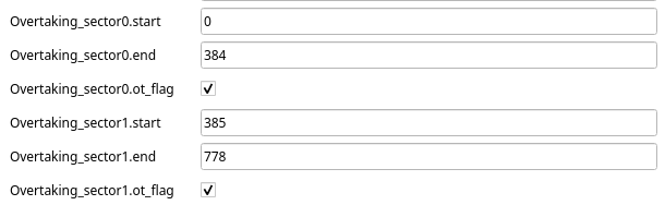RQT’s overtaking sector settings (each sector’s start/end and ot_flag)

Screening the Obstacles to Avoid

Once inside an overtake-enabled sector, of the perceived dynamic obstacles only those satisfying both conditions below remain avoidance targets.

• Within lookahead (15 m) ahead
• Within obs_traj_tresh (2.0 m) laterally of the optimal line

Even with targets present, a trajectory is only generated when all of the following hold.

Condition	Pass criterion
Targets exist (considered_obs)	At least one obstacle passed the filters above
Prediction freshness (prediction_is_fresh)	A GP trajectory prediction arrived within pred_timeout (0.5 s)
Forced trailing off (force_trailing)	The forced-trailing switch, enabled when GP predictions cannot be trusted, is off

If any one fails, the planner never reaches the path-generation stage and no avoidance path is published — a guard against reckless overtaking paths going out when the prediction is uncertain.

The GP predictor cannot produce a trained prediction until the opponent’s trajectory data accumulates to one lap’s worth (cumulative distance ≥ track length). During that period the trajectory topic is not published or force_trailing stays True, and since the lane change node subscribes to this topic as a gate, the car only trails without avoiding. If the data stream is interrupted, the accumulation resets — overtaking activates only after a valid lap’s worth of trajectory has been gathered.

In the video above, the car trails the opponent through its first lap and overtakes into the adjacent lane once measuring is done. You can see that despite ample space on the track, no overtaking trajectory appears while prediction data is insufficient.

2. Choosing the Lane to Take (more_space)

The car evades toward whichever side has more free space. For each obstacle, more_space measures the clearance from the obstacle’s edge to each wall and takes as candidates the sides free by at least the minimum space (min_space), which accounts for the car width and a safety margin.

left_gap  = (left wall clearance) - obstacle's left edge
right_gap = (right wall clearance) + obstacle's right edge
min_space = spline_bound_mindist + width_car/2 + safety_margin

• If only one side is roomy, take it.
• If both are, take the wider one.
• If both are tight, there is no room to pass — do not avoid (return None).

With multiple overlapping obstacles, the passable side is tallied per obstacle. The final direction (preferred_side) is the side satisfying all three:

• More obstacles voted for that side
• That side’s average clearance is wider than the other’s
• That average clearance exceeds the car width

Suppressing Direction Flicker (hysteresis)

If the free space fluctuates slightly every frame, the chosen side can flip left and right, destabilizing the path. To prevent this, the direction only actually changes when the new side persists for consecutive side_switch_frames (10 frames) (_apply_side_hysteresis) — about 0.5 s at 20 Hz, filtering out flips caused by momentary gap fluctuations.

3. Building the d-Profile

Once the side is decided, that lane becomes the target and the avoidance path’s lateral displacement $d$ is drawn. Unlike static avoidance, which placed a single apex point, here the pre-built lane’s $d$ value is followed throughout the obstacle section.

The $s$ axis is unrolled from the car’s current $s$, past the obstacle’s end, to the rejoin point, and the target lane’s $d$ is taken at each $s$. The obstacle section is the $s$ range (start to end) of the predicted opponent trajectory, and a cosine-ease weight $w$ centered on this section shapes the final $d$.

• Entry ramp (back_to_raceline_before): line → lane ($w$: 0 → 1)
• Obstacle section: hugging the lane ($w$ = 1)
• Return ramp (back_to_raceline_after): from the predicted trajectory’s end $s$, lane → line ($w$: 1 → 0)

So the return ramp starts where the predicted opponent trajectory ends. Keeping the entry and return ramp widths separate lets you tune the approach toward the opponent and the return to the optimal line independently.

The entry ramp’s start is fixed at obstacle start − before, but the path is always drawn from the car’s current $s$. So where the car currently sits within the ramp (its $s$ fraction) determines the starting $d$: behind the ramp start, the car departs gently from $d=0$ (the line); already inside the ramp, it starts at the $d$ opened up by that fraction and closes onto the lane sharply within the remaining ramp.

Where the car starts within the ramp is decided jointly by back_to_raceline_before and the trailing distance to the opponent — and their combination determines how smooth the steering is.

If the car is mid-ramp (short trailing distance with a long before), the ramp start lies behind the car, so the path emerges beside rather than beneath the car and a momentarily sharp steering input can occur.

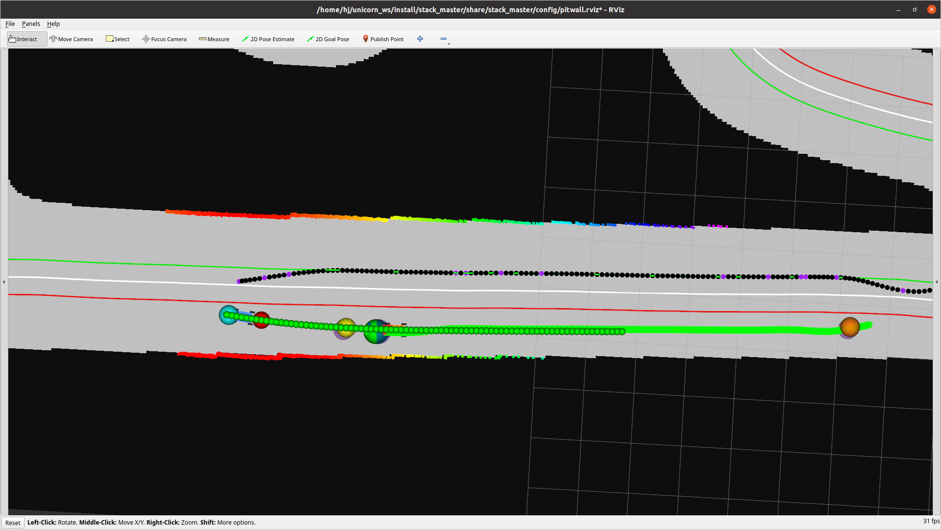The car mid-way into the entry ramp: the ramp starts behind the car, so the path begins beside it

With a short before, the trajectory itself takes a sharp shape, likewise producing abrupt steering.

A short before: the avoidance path bends sharply onto the left lane close to the obstacle

Conversely, a long trailing distance lets the car use the full ramp of a long before and join with smooth steering — but the greater distance to the opponent can work against completing the overtake.

Smooth steering and overtaking success thus trade off against each other, calling for tuning that accounts for track width and the speed difference to the opponent. Thanks to the cosine ease, $d$ itself always joins and leaves the lane seamlessly.

4. Publishing and Debugging

An avoidance path validated to lie inside the track is published and handed to the state machine and the tracking controller. The published topics are below; subscribing in RViz lets you visually check the lanes, the avoidance path, and the validation state.

• /planner/avoidance/otwpnts: the published avoidance path
• /planner/avoidance/merger: the rejoin section — carries both the “obstacle end s” and the “avoidance path end s,” telling downstream modules where to merge back onto the optimal line after the avoidance.
• /planner/avoidance/lane_markers: the pre-built left/right lanes
• /spline_sample_points: the sample points used for the track safety check (any point outside discards the path)

Running It in the UNICORN Racing Stack

The Lane Change Planner is included in race.launch.xml and set as the default overtaking planner, so it runs along with the full driving stack without any extra flags.

unicorn          # enter the conda environment
ros2 launch stack_master race.launch.xml map:=f sim:=true

• map: map name (a folder under stack_master/maps/)
• sim: true for simulation, false on the real car

Tuning with RQT (Dynamic Reconfigure)

All of this planner’s avoidance parameters are declared for dynamic reconfigure, so you can adjust them live in rqt — without restarting the node — and watch how the avoidance behavior changes.

# terminal 1: the driving stack (lane_change is the default overtaking planner)
unicorn
ros2 launch stack_master race.launch.xml map:=f sim:=true

# terminal 2: rqt (must be the same unicorn environment)
unicorn
rqt

Each parameter maps directly to the steps described above. Changes apply to the next frame’s avoidance path with no node restart, so you can watch the behavior shift while viewing the lane markers (lane_markers) and the avoidance path (otwpnts) in RViz.

Parameter	Default	Function
lane_offset	0.35	Distance from the centerline to each lane [m]. Changing it regenerates both lanes immediately; larger hugs the walls and passes the opponent wider, smaller passes closer to the optimal line (step 0).
back_to_raceline_before	3.0	Entry-ramp width onto the lane ahead of the obstacle [m]. Larger joins the lane earlier and more gently (step 3).
back_to_raceline_after	3.0	Return-ramp width back to the optimal line past the obstacle [m]. Tunes return gentleness independently of entry (step 3).
obs_traj_tresh	2.0	Only obstacles within this lateral distance of the optimal line are considered [m] (step 1).
spline_bound_mindist	0.3	Clearance value setting both the minimum space required when choosing a side and the lower bound on wall proximity [m] (step 2).
safety_margin	0.1	Safety margin around the car and obstacles [m] (step 2).
evasion_dist	0.3	Clearance secured beside the obstacle [m].
max_evasion_start_offset	0.8	Upper bound: if the lateral jump demanded at the path start exceeds this, the path is discarded [m] (step 4).
pred_timeout	0.5	Freshness criterion: a GP prediction must have arrived within this time for overtaking to start [s] (step 1).

Driving Example

Even on a narrow track (map_test), the car overtakes the opponent into the adjacent lane stably.

Wrap-up

This post walked step by step through the Lane Change Planner, which takes two pre-built lanes flanking the centerline as avoidance targets, merging onto the free lane around an obstacle and then returning to the optimal line. The flow runs lane building → overtake gate (ot_sectors, GP prediction freshness) → side decision (hysteresis) → cosine-ease d-profile → validation and publishing, with lane_offset and the entry/return ramp widths (back_to_raceline_before/after) as the key tuning points. For static obstacles, see Static Obstacle Avoidance.