Particle Filter Localization — Measurement Model

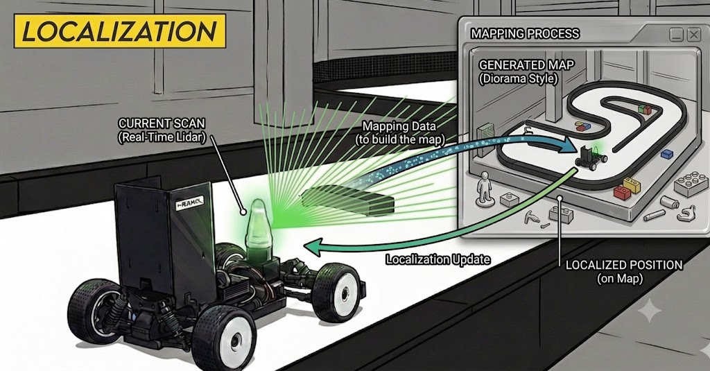
In the previous motion model, we spread particles over the map by as much as the odometry uncertainty. Now it’s time to pick out, among the many scattered particles, which one is actually at my position. The tool for this is the Measurement Model, also called the Sensor Model.

If the motion model is the process of guessing ‘roughly where have I come to?’, the measurement model is the process of scoring ‘how well does the scene in front of me match my guess?’ The measurement model predicts the virtual scan each particle would observe assuming it is at its own pose, and compares it to what the real robot observed. The more similar the two, the higher the probability that particle is the true position, so it gets a high weight; if they differ, the weight is cut. Only through this can the following resampling step let the particles near the true position survive and cluster.

So how do we implement this measurement model?

1. The Limit and Compute Bottleneck of Virtual-LiDAR Matching (Raycasting)

The most intuitive sensor model — and the one our stack adopts as its main approach — is raycasting: from each particle’s virtual pose, shoot virtual rays toward the occupancy grid map and compute distances.

The raycasting we commonly use must scan grid cells one by one with Bresenham or DDA to find the walls, so it is very heavy.

• Number of particles: $M$ (e.g., 1000)
• Number of LiDAR rays: $N$ (e.g., 360 per channel)
• Total cost: $O(M \times N)$ raytracing operations every loop

This is incomparably heavier than a motion-model update. On a single CPU thread, securing real-time performance (at least 20 Hz) is nearly impossible.

How to Run Heavy Raycasting in Real Time

Fortunately, raycasting is perfectly independent per particle and per ray — an embarrassingly parallel structure. So if you have a GPU, you can process raycasting for thousands of particles at once (e.g., a CUDA build on an NVIDIA Jetson) and greatly raise the compute speed.

Of course, a GPU is not mandatory. You can run it on CPU alone, and if you have memory to spare, you can secure real-time performance on CPU too by looking up a look-up table (LUT) of precomputed results instead of scanning the grid every time. We look at various optimizations — including LUT-based ones — in the next section.

Aside: Scoring Without Raycasting (AMCL’s Distance Transform)

Raycasting is heavy because of ‘traversing inside the map to find walls.’ ROS’s standard package AMCL (Adaptive Monte Carlo Localization) also offers a Likelihood Field approach that removes this step entirely. When loading the map, it precomputes — via a Distance Transform — the distance from each cell to the nearest wall, and at runtime, instead of shooting virtual rays, it only projects the end points of the real scan onto the map and reads that distance in $O(1)$. It’s fast on CPU alone without a GPU, but the precise distance-field table eats a lot of memory and it is relatively vulnerable to dynamic obstacles not in the map. We use raycasting as our main method, exploiting GPU parallelism, and just keep in mind that “there’s also a way to make a score without raycasting.”

In the demo below, see how a likelihood field — precomputed by a distance transform — is used to score by projecting only the real scan’s end points, with no raycasting.

2. Various Raycasting Techniques and Their Trade-offs

Virtual-LiDAR matching isn’t only the Bresenham method of scanning cells one by one. Depending on hardware/memory constraints, various optimizations apply.

• Bresenham / DDA — inspects visited cells one by one. Needs no precomputation, only map data, but is compute-heavy and grid-resolution limited.
• Ray Marching (Sphere Tracing) — precomputes a distance-transform map once. At each position, jumps across empty space by the minimum distance to a wall, speeding up the search.
• CDDT / PCDDT — builds per-direction look-up tables, compressed. Queries two and interpolates, and prunes to reduce computation.
• Giant LUT — bakes results for all $x, y, \theta$ in advance. A single $O(1)$ lookup — the fastest — but the entries grow exponentially and consume enormous RAM.
• Analytic (line segments) — inspects a list of line segments directly without a grid. Exact precision regardless of grid resolution.

In the demo below, see how the various raycasting techniques find walls on a grid map and get a feel for each method’s characteristics.

3. Weight Computation

Once you’ve built each particle’s virtual scan, it’s time to compare with the real LiDAR scan and score. Plug the difference between each particle’s virtual scan and the real scan into a Gaussian to get a probability.

\[p(o_t \mid \bar{x}_t^i) = \frac{1}{\sigma\sqrt{2\pi}}\, e^{-\frac{(o_t - r^i)^2}{2\sigma^2}}\]

Over multiple rays ($k$), multiply each ray’s probability to get the particle’s final weight.

\[w^i \propto \prod_k \exp\!\left(-\frac{\left(z_k^{\text{obs}} - z_k^{\text{exp}}\right)^2}{2\sigma^2}\right)\]

The meaning is simple: the closer a particle’s expected scan is to the real observation, the exponentially larger the weight it receives.

In the demo below, see how the Gaussian score is assigned from the error between the expected distance and the real observation, and how the scores of multiple rays multiply into a single particle’s final weight.

4. Resampling & Final Pose

Once weights are computed, perform resampling — keep high-scoring particles and discard low ones. Typically you sample uniformly at $1/M$ intervals over the cumulative-weight distribution. This way high-weight particles are naturally selected multiple times and replicated, while near-zero particles are culled.

After resampling, the surviving particles cluster densely around the real robot position. You then either pick the most frequent particle position or compute the expectation of the whole distribution to fix the robot’s final estimated pose.

How to use

Start particle filter localization on a saved map on the real car.

ros2 launch stack_master localization.launch.xml map:=<map_name> localization:=pf

The sensors/mux (low_level) and the map_server come up together, and the particle filter’s pose estimate is published to /car_state/odom through the EKF.

Set the initial pose with RViz’s 2D Pose Estimate (/initialpose) — it re-initializes the particles around the clicked pose.

Wrap-up

The measurement model is, in the end, the core process of evaluating many hypotheses from LiDAR data (weighting), distilling only the good ones (resampling), and deriving the final answer.

We made scoring by virtual LiDAR (raycasting) our main approach. Raycasting is heavy but perfectly parallel, so with a GPU you accelerate it as-is, and without one you can push it on CPU with a LUT — it hardly cares about the hardware. In the end, choosing an algorithm goes beyond grabbing a famous method: you must weigh it together with the hardware architecture and the limits of your compute budget.

The particle filter is, as shown, simple and intuitive in code, which makes it easy to understand and work with. That said, under actual high-speed driving its pose estimate turned out somewhat unstable. So the next post introduces Cartographer-based pose estimation to make up for that.

References

• mit-racecar/particle_filter — the base particle-filter implementation
• kctess5/range_libc — raycasting (Bresenham · Ray Marching · CDDT · GLT) library
• https://www.youtube.com/watch?v=SRBdpoPl57Q