Frenet-based Tracking: Linking the Opponent Across Time

Intro — The Problem We’re Solving

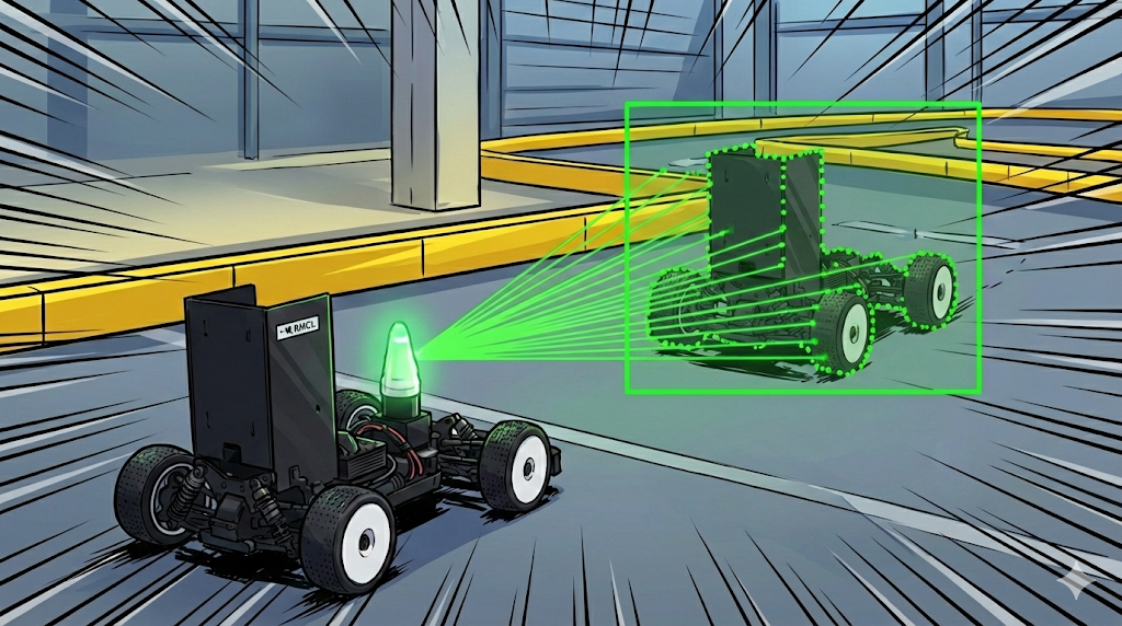
In autonomous racing, while my car (ego) drives the track it must know, in real time, “is there another object (an opponent car) ahead of me? If so, where, and how fast is it moving?” Only then can it decide whether to overtake, follow, or avoid.

Perception is responsible for this, in two stages.

1. Detection — from a single LiDAR scan “right now,” find object blobs and represent them as boxes. → node detect (perception/src/detect.cpp) — the topic of the two previous posts (Detection & Clustering · Feature Extraction)
2. Tracking — stitch the per-frame detected boxes along time, assign a unique ID to the same object, estimate velocity, and classify static/dynamic. → node tracking (perception/scripts/multi_tracking.py) — the topic of this post

One-liner: Detection = “what’s visible now” (a snapshot), Tracking = “is that the same one as before, and where is it heading” (the flow of time).

2. What Is Tracking?

2.1 Why Detection Alone Isn’t Enough

Detection is independent per frame. The box detected at frame t and the box at frame t+1 — it doesn’t know whether they’re the same object. So from detection results alone:

• The ID changes every frame (temporary numbers 0,1,2… assigned each time)
• You can’t know velocity (a single snapshot doesn’t show motion)
• It’s noise-prone (a one-frame false blink comes through as-is)

2.2 What Tracking Does

Tracking stitches consecutive frames to produce:

Function	Description
Data Association	match this frame’s detection to whichever object was being tracked
State Estimation	smooth the position with a Kalman filter and estimate velocity
ID management	keep a persistent ID for the same object; delete it a while after it disappears
Static/Dynamic classification	tell static objects (walls, cones) from a moving opponent (dynamic)

That is, tracking’s output is a meaningful state like “object #5 is dynamic (an opponent), at s=42 m, d=0.3 m, approaching at 3.1 m/s longitudinally.”

3. The Full Pipeline at a Glance

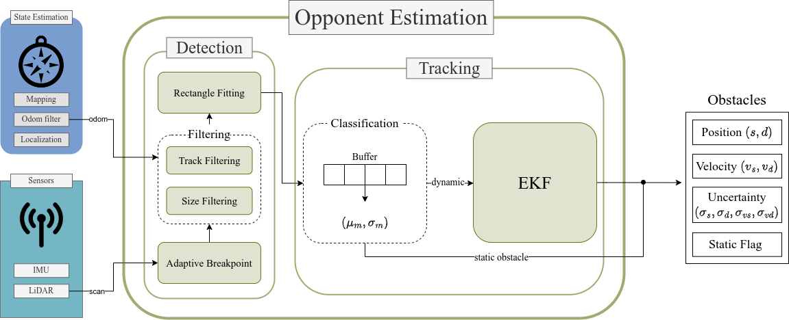
• Inputs: LiDAR /scan, track reference line /global_waypoints_scaled, ego state /car_state/odom(_frenet)
• Intermediate: /detect/raw_obstacles — detection’s instantaneous detections (position only)
• Final: /tracking/obstacles — tracked dynamic obstacles (with ID·velocity), /tracking/raw_obstacles — static/unclassified

4. (Recap of the Two Previous Posts) What Detection Hands to Tracking

What happens in detect.cpp

Node name detect. On each timer tick (rate_detect, default 10 Hz), timerCallback() runs in this order.

Sections 4.1–4.5 below are a recap — compressing only what’s needed for tracking — of content already covered in detail in the two previous posts (Detection & Clustering · Feature Extraction). If you’ve read them, jump straight to 4.5 and section 5. For details — the derivation of the range-adaptive threshold D_max, dual-stage clustering, rectangle-fitting checks — see the two earlier posts.

4.1 Scan → Map Coordinate Conversion

Convert each LiDAR beam (r, angle) to a laser-frame point (x, y), then via tf (map ← laser) into map-frame coordinates. (code: clustering())

4.2 Removing Off-track Points (Map Filter)

Using a mask made by eroding the preloaded map image, keep only “points inside the track” (GridFilter_.isPointInside). This filters out beyond-the-wall and track-boundary noise, leaving only opponent candidates. (see Grid Filter for details)

4.3 Adaptive Breakpoint Clustering

Sweeping the points, split by the distance between adjacent points. The key is that the distance threshold isn’t fixed but grows in proportion to range — since LiDAR points spread apart with distance:

d_max = curr_range * sin(dφ) / sin(λ - dφ) + 3σ

Closer than d_max → same cluster; otherwise attach to a nearby existing cluster (within new_cluster_threshold_m) or start a new one. Finally, clusters with too few points (min_size_n, default under 10) are dropped.

4.4 Feature Extraction — L-shape Fitting

A car/obstacle usually appears as an L-shape to LiDAR. Sweeping 90 candidate angles (0°–90°), pick the angle where the points best hug two rectangle edges by a score (∑ 1/distance), estimating the box center · size · rotation (theta). If the size exceeds max_size_m, it’s judged not an opponent and dropped (checkObstacles).

4.5 What Passes to Tracking (Published After Frenet Conversion)

Each box center (x, y) is converted to (s, d) via GetFrenetPoint() and published as /detect/raw_obstacles (ObstacleArray).

Limits of the detection output (important): the id in this message is a temporary number valid only within that frame (0,1,2…), and velocity (vs,vd) and static/dynamic info are not filled in. It’s an instantaneous snapshot with only position (s_center,d_center) and size (size). Adding time-axis information to this is the next tracking stage.

5. The Tracking Stage — multi_tracking.py

Node name tracking. It subscribes to /detect/raw_obstacles and, on each timer tick (rate_tracking), timer_callback() runs predict → update → publish.

5.1 Data Association (Nearest-Neighbor)

Among this frame’s detections, match the one closest to the predicted position of each tracked object (verify_position → get_closest_pos). Distance is in Frenet:

dist = hypot( normalize_s(Δs), Δd )      # s wraps, accounting for the track's seam (one lap)

Pick the nearest among candidates inside the gate max_dist. Dynamic objects use the predicted position and widen the gate by aggro_multiplier× to follow better. On repeated match failures, the TTL (time-to-live) is decremented; at TTL 0 the object is deleted. A “new detection” matched to nothing gets a new persistent ID (self.current_id, ever-increasing).

5.2 Frenet EKF — State and Model

Each object gets its own Extended Kalman Filter (EKF) (Opponent_state). The state vector is:

\[X = [\,s,\; v_s,\; d,\; v_d\,]^T\]

A constant-velocity model is used on the Frenet frame.

\[\begin{aligned} s_{k+1} &= s_k + v_s\,\Delta t, &\quad v_{s,k+1} &= v_s \\ d_{k+1} &= d_k + v_d\,\Delta t, &\quad v_{d,k+1} &= v_d \end{aligned}\]

A control input $u$ injects a little prior: $-P_d\,d$ and $-P_{vd}\,v_d$ reflect the tendency of an object to return to the lane center ($d=0$), and (when the object is briefly lost) $P_{vs}(v_{target} - v_s)$ reflects the tendency to follow the track’s reference speed.

Why an “E”KF, not a plain KF? The model itself is linear (constant velocity), but when $s$ completes a lap it must wrap from track_length back to 0 (the seam) — a nonlinear step (normalize_s). This wrap has to be handled in the measurement/residual functions (hx, residual_h), so the EKF form (filterpy.ExtendedKalmanFilter) is used.

As summarized in the previous Feature Extraction post, the orientation (θ) and shape that detection obtains from rectangle/L-shape fitting are not passed to tracking — they’re only for RViz marker visualization. The tracker receives only the box center (s, d), and velocity comes from the frame-to-frame difference of that center.

The measurement feeds in the (s, d) given by detection together with the velocity from frame-to-frame differences (update()):

z = [ s_meas,  vs(=Δs·rate, seam-corrected),  d_meas,  vd(=Δd·rate) ]

Absurd velocities (vs outside −1–8 m/s) are treated as spikes; the filter is re-initialized to prevent divergence.

In the demo below, you can interact with how an opponent is tracked on the Frenet frame — repeating predict → update while keeping the ID and estimating velocity.

5.3 Static / Dynamic Classification (Voting)

For each object, compute the standard deviation std_s, std_d of recent measurements (isStatic). If the position barely changes (both under min_std), cast a “static vote”; if it changes a lot (over max_std), reset. A static-vote ratio ≥ 0.5 classifies it as static.

• Static → fix the position to its average (walls, cones, etc.)
• Dynamic → treat as an opponent, track with the EKF above, estimate velocity
• Unclassified → not enough measurements yet (min_nb_meas) (judgment deferred)

5.4 Velocity Smoothing & Publishing

The estimated longitudinal/lateral velocities are smoothed with a length-5 moving average (vs_filt, vd_filt) before publishing. The publish branch (publishObstacles):

• Dynamic and with small enough position covariance (P[0][0] < var_pub) only → /tracking/obstacles (trustworthy opponents)
• Static/unclassified → /tracking/raw_obstacles

Here each Obstacle message is filled with persistent ID, velocity (vs,vd), covariance (s_var…), static flag (is_static), and Cartesian coordinates (x_m,y_m).

6. What to Check, and How, in a Real Run

After building/running (e.g., ros2 launch stack_master race.launch.xml sim:=true map:=f), you can inspect the topics directly in a terminal.

6.1 Key Topics

Topic	Type	Meaning
/detect/raw_obstacles	ObstacleArray	detection’s instantaneous detections (position only, temp ID, no velocity)
/tracking/obstacles	ObstacleArray	tracked dynamic opponents (persistent ID · velocity · covariance)
/tracking/raw_obstacles	ObstacleArray	static/unclassified obstacles
/tracking/static_dynamic_marker_pub	MarkerArray	markers for RViz visualization
/tracking/latency	Float32	(measure mode) processing frequency

6.2 Inspecting Topic Values Directly

# check tracked opponents — velocity and target id are visible here
ros2 topic echo /tracking/obstacles

# compare with (instantaneous) detection
ros2 topic echo /detect/raw_obstacles

6.3 How to Read the Obstacle Fields of /tracking/obstacles

Field	Meaning	What to look for
id	tracked target ID	for the same car, the number persists across frames (detection changes every time)
vs	longitudinal velocity (s, m/s)	+ when the opponent approaches, smoothed by moving average
vd	lateral velocity (d, m/s)	lane change / side-to-side motion
s_center, d_center	Frenet position	“how many m along the track, how many m off center”
x_m, y_m	corresponding Cartesian position	real coordinates in RViz/map
s_var, vs_var, d_var, vd_var	Kalman covariance	larger = more uncertain (small is trustworthy)
is_static	static flag	opponents in /tracking/obstacles are False
is_visible	currently in view?	False if occluded (kept by prediction)
size	box size	value from the detection L-shape

How to see the detection-vs-tracking difference with your own eyes: echoing /detect/raw_obstacles, vs,vd are 0 and the id changes every frame. In contrast, /tracking/obstacles keeps the same car’s id and stamps real velocity values into vs,vd. This contrast best shows “what tracking adds.”

6.4 Seeing It via RViz Marker Colors

Displaying /tracking/static_dynamic_marker_pub in RViz shows the classification state by sphere-marker color.

• 🟢 green = static obstacle
• 🔵 blue = dynamic opponent
• 🔴 red = unclassified (not yet judged)

Objects that are in front (isInFront) or have small covariance (high confidence) are drawn as larger markers.

Wrap-up

1. Frenet coordinates (s, d) are a frame that “unrolls” a winding track — making motion on the track simple.
2. Detection (detect.cpp) finds boxes from a single LiDAR scan via clustering + L-shape, emitting a position-only instantaneous snapshot (/detect/raw_obstacles).
3. Tracking (multi_tracking.py) uses NN association + a Frenet EKF (state [s,vs,d,vd]) + static/dynamic classification + TTL/persistent IDs to emit a meaningful state (/tracking/obstacles).
4. At runtime, verify behavior via the id·vs/vd·is_static of ros2 topic echo /tracking/obstacles and the RViz marker colors.

References

• Previous posts: Detection & Clustering · Feature Extraction
• Code: perception/scripts/multi_tracking.py, perception/src/detect.cpp (unicorn-racing-stack)
• Message definition: f110_msgs/msg/Obstacle.msg
• State estimation: filterpy ExtendedKalmanFilter
• Background: datmo (kostaskonkk) · TU Delft thesis