Particle Filter Localization — Motion Model and Resampling

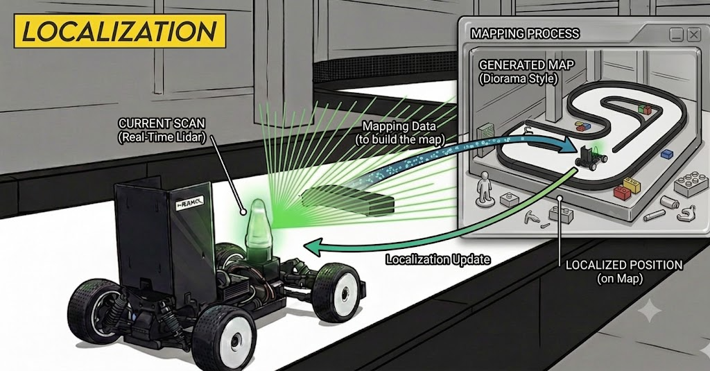
The first problem an autonomous car or robot must solve to drive on its own is knowing “where am I on the map right now.” But real-world sensors have resolution limits and noise, and motors and drivetrains never move perfectly either, due to wear and control noise.

This post looks at the Particle Filter — the algorithm we chose to handle this inherent uncertainty — and details the Motion Model and Resampling, the first pieces of the localization stack.

1. What Is a Particle Filter?

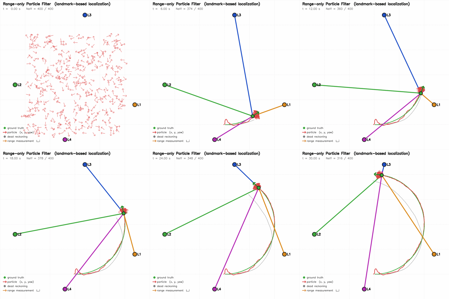
In one sentence, a particle filter is an algorithm that “scatters many virtual robots (particles) over the map, keeps only the particles most consistent with the real sensor data, and narrows down the position.” The key is representing the probability distribution non-parametrically — with a finite set of samples (particles) rather than a complex analytic formula.

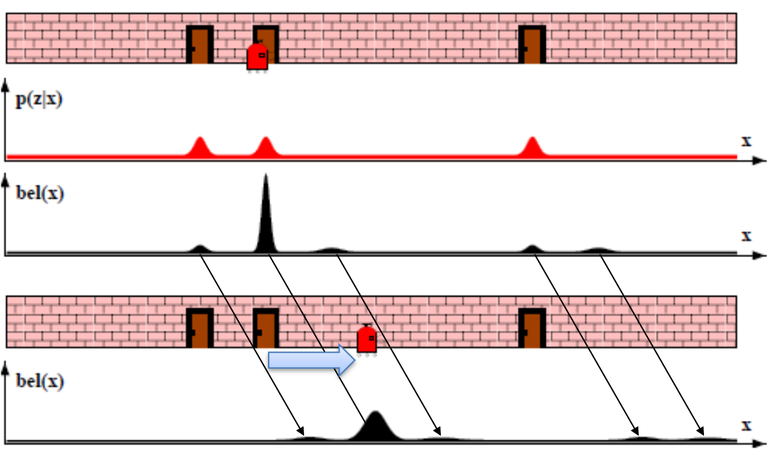
A particle filter is built from a Motion Model that predicts the robot’s motion and a Measurement Model (Sensor Model) that evaluates sensor observations. While driving, it endlessly repeats these three steps.

1. Motion update (Motion Model) — move every particle based on the robot’s control input / odometry.
2. Weighting (Sensor Model) — at each particle’s pose, generate a virtual sensor scan, compare it to the real LiDAR observation, and assign a weight by the posterior probability.
3. Resampling — replicate high-weight particles into several copies and kill off low-weight ones, forming a new particle set.

One important property: a particle filter can find the answer even starting with no idea of the initial position (Global Localization). Even if particles are spread uniformly across the whole map at first, they gradually cluster around the true position as the robot moves and gathers sensor data.

This post covers the Motion Model and Resampling of these three steps. (The sensor model continues in the next post.)

2. Motion Model: To Move Particles, You Need ‘Dynamic Information’

Let’s dig into the first step, the motion model. What it does is simple — figure out how much the robot moved since the previous frame, and move every particle by that much. Just because the particle filter is strong at global search doesn’t make scattering thousands every frame with no hint wise; it’s wasteful. So you must concentrate particles in the region the robot is likely in, using the dynamic information “the robot moved roughly this much.”

There are several ways to obtain this dynamic information.

• Differentiate the previous pose — divide the difference of recently estimated poses by time to get velocity. Needs no extra sensor, but the estimation’s own noise and latency ride directly on the velocity.
• Use extra information (sensors) — get velocity/angular velocity directly from separate sensors like an IMU or wheel encoders.

Simply, you can obtain this via the VESC (motor controller)’s wheel odometry. From the motor rotation speed the VESC reports, we get the vehicle’s forward speed, and combining it with the steering angle we get the angular velocity (yaw rate) — yielding the body-frame displacement (forward · rotation), “the car moved roughly this much since the previous frame,” in real time. This becomes the motion model’s control input, moving every particle by that much, so the particle filter efficiently concentrates its hypotheses in the likely region instead of searching the wrong space.

3. Odometry Uncertainty and Process Noise

A real race car does not trace its trajectory exactly as the odometry numbers say. In racing especially, odometry accuracy degrades badly for several reasons.

• Slippage — inevitable between tire and road at high speed and in sharp turns.
• Wheel spin on a hard launch — the wheels spin faster than the actual motion, so the encoder overestimates the traveled distance.
• Wheel lock on hard braking — even if the wheels stop, the body slides on by inertia, so the encoder underestimates the traveled distance.

So when implementing the motion model, you must not use the deterministic approach of simply adding the odometry displacement to the previous particle pose. When moving particles, you must sample independent Gaussian noise and add it explicitly.

This noise is the device that reflects, in the particle distribution, the uncertainty that “to the extent the odometry can’t be trusted, spread the particles over the range where the vehicle’s true position could be.”

In the demo below, adjust the noise parameters (MOTION_DISPERSION_X/Y/THETA) yourself and see how particles spread from a single pose.

4. The Key Detail: Tuning the Uncertainty Parameter and Particle Behavior

The Gaussian-noise parameter of this motion model reflects the uncertainty of the wheel odometry. How you set it determines the spread radius of the particles right after a motion update.

1) Tuned too small (Underestimation)

• Symptom — the filter over-trusts the odometry. Even after a motion update, particles don’t spread; they move as a single tight point.
• Problem — the moment any slip occurs in a corner, the true position (ground truth) escapes the particle distribution entirely. Then even after sensor matching and resampling, not a single particle survives near the answer, so the filter points somewhere completely wrong and diverges.

2) Tuned too large (Overestimation)

• Symptom — the filter distrusts the odometry. On every motion update, particles spread excessively into places they never went.
• Problem — with particles too scattered, a wide range shares the weight little by little at resampling. In segments where sensor matching can’t decisively concentrate the weight, the particle centroid wobbles around, producing a noisy output that feeds unstable pose to the control stack.

The point, in the end, is that you must quantify your own odometry’s uncertainty and carry it as this parameter. The trouble is that the right value varies with the driving environment (surface, corner characteristics) and with your own driving style and tuning. So no single fixed value covers every situation, which makes choosing it tricky in itself. Fundamentally, the more accurate the base odometry, the smaller you can keep this uncertainty — which is an advantage.

5. Resampling: Cluster, Then Spread Again

The particles spread by the motion model receive weights in the sensor model (next post) by comparison with the real LiDAR observation. Resampling is the step that reflects these weights back into the actual particle count.

The key is weighted resampling (sampling with replacement proportional to weight). Higher-weight particles are replicated several times into the next generation; lower-weight ones die out.

# resample N with replacement, proportional to the weights (p=weights)
proposal_indices = np.random.choice(self.particle_indices, self.MAX_PARTICLES, p=self.weights)
proposal_distribution = self.particles[proposal_indices, :]

Here the motion model and resampling interlock as a pair. Because resampling draws with replacement, a high-weight particle survives as several copies at the exact same coordinate. Left like this, particle diversity vanishes (sample impoverishment) — but the very next step’s motion-model noise re-scatters these copies, restoring diversity. That is, it repeats “cluster near the answer by resampling → spread again by motion noise” every frame, narrowing down the position. This is another reason we said the noise parameter must be tuned “just enough to barely enclose the answer” — too small and the copies freeze in a clump, too large and the hard-won particles scatter again.

Two details of our code:

• We resample unconditionally every frame (no adaptive resampling with an effective-sample-size threshold).
• It’s multinomial resampling based on np.random.choice, and the actual execution order is resample → motion → sensor (a slightly different arrangement from the conceptual three-step order).

Wrap-up

The particle filter’s motion model is, in the end, the process of admitting real-world uncertainty and cleverly spreading particles by as much as the odometry error. And when resampling gathers the particles back around the answer, motion noise re-scatters them — this cycle repeats every frame.

How these spread-and-gathered particles meet the real LiDAR scan to earn weights and finally converge — and the optimization techniques that resolve the compute bottleneck in that process — is continued in Particle Filter — Measurement Model.

References

• mit-racecar/particle_filter