Static Obstacle Avoidance: The Static-Obstacle Evasion Spline
Related code: planner/spliner/spliner/static_avoidance_node.py
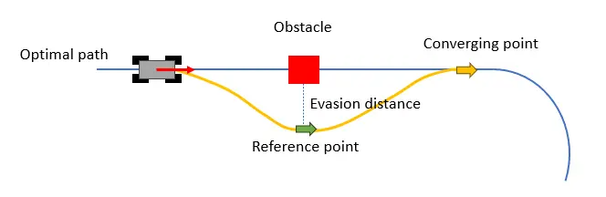
static_avoidance_node.py (node name static_avoidance_planner) generates, at 20 Hz, an avoidance trajectory that briefly leaves the optimal line (the IQP global line) to dodge a detected static obstacle and then returns. It receives a single obstacle designated by the upstream behavior/state machine and publishes a short detour line starting from the vehicle’s current pose.
The core idea is to handle the evasion line in the Frenet coordinate frame. $s$ is the distance traveled along the track and $d$ is the lateral distance from the reference line — the optimal line being followed becomes the $d=0$ reference. The evasion line is expressed as a profile that grows the lateral displacement $d(s)$ out to an apex beside the obstacle and brings it back to 0.
Here $p_{race}$ is a point on the optimal line and $n$ is the unit normal. With this formulation, deciding which side to pass and by how much becomes a one-dimensional problem of choosing a few $d$ values, and staying on the track becomes the box constraint $-w_{right} \le d \le w_{left}$. (This is the same structure as gb_optimizer’s alpha parameterization.)
When converting the generated $(s,d)$ points into an actual $(x,y)$ curve, not only each point’s position but also the direction of travel (tangent) at that point is specified, interpolating with BPoly.from_derivatives. Since the direction is continuous (C1), the result is a smooth curve the vehicle can actually follow.
Architecture
1
2
3
4
5
6
7
8
9
10
11
12
13
14
15
/behavior_strategy            (obstacle of interest)
/car_state/odom_frenet        (ego Frenet state s, d)
/car_state/odom               (ego cartesian pose x, y, yaw)
/global_waypoints             (FrenetConverter init, gb_vmax / gb_max_s)
/global_waypoints_scaled      (optimal line = d=0 reference)
        |
        v
static_avoidance_node.py  ─  do_spline()  (20 Hz)
        |
        | publishes /planner/avoidance/otwpnts
        |   └─ remapped to /planner/avoidance/static_otwpnts in race.launch.xml
        | publishes /planner/avoidance/markers          (visualization)
        | publishes /planner/avoidance/spline_samples   (debug bounds-check markers)
        v
state machine / tracking control (Pure Pursuit, etc.)
| Step | Function | Role |
|---|---|---|
| 1 | loop / behavior_cb | Select the obstacle of interest + forward-distance gate |
| 2 | _more_space | Decide evasion side and depth $d_{apex}$ |
| 3 | do_spline (Frenet) | Build the d-profile (apex + return points) |
| 4 | do_spline (BPoly) | Turn it into an (x,y) curve with a tangent-matched spline |
| 5 | savgol / quad-ease | Smoothing + merging back into the optimal raceline |
| 6 | is_point_inside | Track-boundary safety check / discard |
1. Selecting the Obstacle of Interest and the Distance Gate
loop() runs at 20 Hz and calls do_spline() whenever there is an obstacle of interest. The obstacle of interest is the first entry of overtaking_targets in /behavior_strategy, taken by behavior_cb; only when that obstacle is static (is_static == True) does this node proceed to generate an avoidance path.
Right after entering do_spline(), if the obstacle is already at close range ahead (under 0.5 m), it is too late to evade and an empty path is returned.
1
2
pre_dist = (obs.s_center - cur_s) % track_length   # forward s-distance to the obstacle
pre_dist < 0.5 m            → return empty path (too close ahead)
2. Deciding the Evasion Side and Depth (_more_space)
The car evades toward whichever side has more free space. On the Frenet $d$ axis, the remaining clearance from the obstacle’s edge to each wall is computed, and only sides with at least the evasion margin free are candidates.
1
2
3
4
pos_gap = gb_wp.d_left  - (obstacle.d_center + obs_radius)   # +d = LEFT wall clearance
neg_gap = (obstacle.d_center - obs_radius) + gb_wp.d_right   # -d = RIGHT wall clearance
min_space = evasion_dist + spline_bound_mindist   # = 0.65 + 0.2 = 0.85 m
→ if only one side qualifies, take it / if both, take the wider one
Once the side is decided, the evasion depth $d_{apex}$ is set evasion_dist further out from the obstacle’s edge, with two clamps.
1
2
3
d_apex = (obs.d_center ± obstacle.size/2) ± evasion_dist
clamp 1: never cross the optimal line (d=0) to the opposite side
clamp 2: never exceed the track walls (d_left / d_right)
Thanks to these, the apex always stays on the same side as the line and inside the walls.
3. Building the d-Profile (Apex + Return Points)
The evasion profile is composed of a few points in Frenet: one apex point beside the obstacle, followed by return points that decrease $d$ linearly from $d_{apex} \rightarrow 0$ over the return segment.
1
2
3
4
post_dist = clamp(pre_dist, post_min=1.5, post_max=5.0)   # distance used for the return
N = post_dist // sampling_dist + 1                         # number of return points
point 0 :  s = obs.s_center,                       d = d_apex
point i :  s = obs.s_center + post_dist·(i+1)/N,   d = d_apex·(1 - (i+1)/N) → 0
The output of this step is not yet a finished $(x,y)$ curve — it is a sequence of $(s,d)$ points that swell out to the apex and come back to 0 relative to the line.
4. The Tangent-Matched Spline (BPoly.from_derivatives)
After converting the $(s,d)$ points to $(x,y)$ with the FrenetConverter, the current vehicle position is prepended to the point list and the current vehicle heading to the tangent list. For the evasion points’ tangents, the optimal raceline heading psi_rad at each location is used.
1
2
3
points   = [ (cur_x, cur_y),  apex,      post_1,    ... ]
tangents = [ cur_yaw,         psi(apex), psi(post_1), ... ] × spline_scale
samples  = BPoly.from_derivatives(cumulative distance, points⊕tangents)   # x and y separately
The curve departs in the direction the vehicle is currently facing, and at the apex and return points it runs parallel to the line. spline_scale (default 0.8) scales the tangents — that is, how long each point holds its direction — and larger values produce larger turning radii.
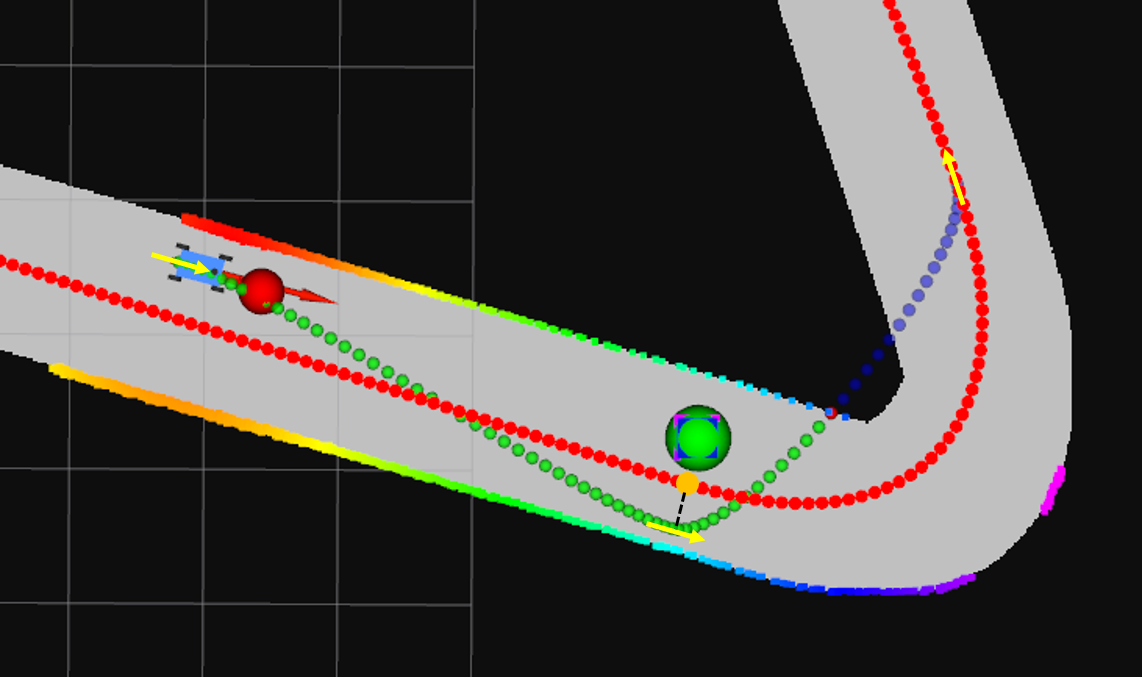 Connecting the points almost straight, relying on position with little heading influence (spline_scale = 0.5)
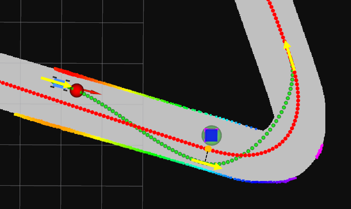 Holding heading moderately, smoothly joining the apex and the convergence point (spline_scale = 1.0)
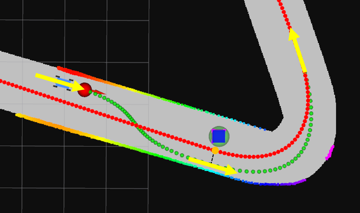 Holding heading too long near the apex and convergence point, swinging out unnecessarily wide (spline_scale = 2.0)
5. Smoothing and Merging Back into the Optimal Line
The spline result is polished once more. A Savitzky–Golay filter straightens the curve while pinning both endpoints (the vehicle’s current pose and the last return point) so the ends do not kink at the filter boundary, and the tail merges into the global line progressively with quadratic weights. In the merge segment the global line’s weight grows along a quadratic curve (quad-ease), so the evasion line converges gently onto the optimal line. After the return points, 100 global waypoints are appended as-is so the path continues along the optimal line after the evasion ends. This step keeps the tracking controller from making abrupt direction changes at the seam between the evasion line and the raceline.
6. Track Safety Check and Discard
Finally, the node verifies the generated path is actually drivable. Every sample point is checked against the map filter (is_point_inside); if even one lies outside the track, the entire avoidance path is discarded (danger_flag → return an empty array). This is a real-time safety guard executed every frame at runtime.
If no evasion line appears, it was most likely discarded at this step. A narrow track or a large
evasion_distpushing the apex too close to the wall are the common causes — checking the/planner/avoidance/spline_samplesmarkers to see which points left the track narrows down the cause.
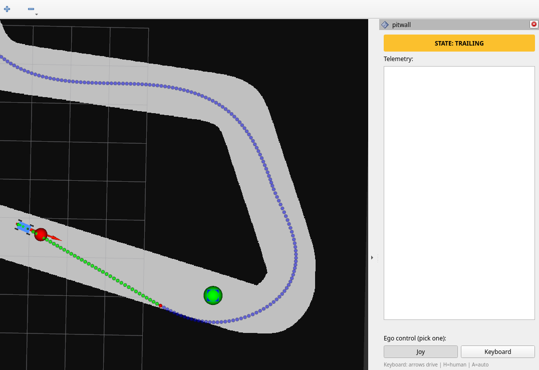 Generated sample points being screened by the map filter (green: pass / red: fail)
Extension: Same Engine, Different Target Points
The skeleton so far — pick target points in Frenet, connect them smoothly with a tangent-matched spline, and screen with a track check — is not used only for static avoidance. Changing what the target points are in steps 2–3 yields different planners.
| Target points | Node |
|---|---|
| The d value of the adjacent lane | change_avoidance_node |
| A rejoin point on the line | recovery_spliner_node |
| A human-clicked pose | start_spline_node_v2 |
Wrap-up
This post walked through static_avoidance_node step by step: when a static obstacle appears on the optimal line, it defines an evasion profile with an apex and a few return points in the Frenet frame, builds a smooth $(x,y)$ curve with a tangent-matched spline (BPoly), and guarantees safety with a track-boundary check. The evasion side/depth (evasion_dist) and curve shape (spline_scale) are the key tuning points, and swapping only the target points extends the same skeleton into other planners — lane change, recovery, and manual start.