Frenet Coordinates: Treating a Curved Track Like a Straight Line

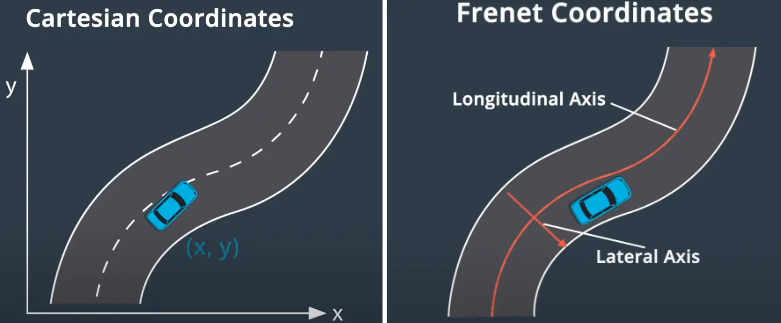
To reason about an opponent’s position and motion in a race, we need a coordinate frame. But a track is not a straight line — it’s a winding curve, and with the usual Cartesian coordinates $(x, y)$, intuitive questions like “ahead or behind?” and “left or right of center?” turn out to be surprisingly awkward to answer. This post covers the Frenet coordinate frame $(s, d)$, which treats a curved track as if it were straightened out, along with the conversions to and from Cartesian coordinates.

1. What Is the Frenet Frame?

1.1 The Inconvenience of Cartesian $(x, y)$

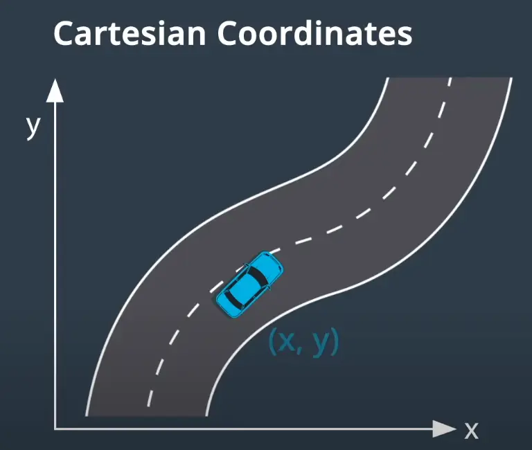
We usually express position as $(x, y)$ on a map. But a track is a winding curve, not a straight line. On a curved track, answering “is the opponent ahead of me or behind?” or “how far left/right of the track center am I?” in $(x, y)$ forces you to keep accounting for the curve’s direction at every instant — very cumbersome.

1.2 The Idea Behind Frenet $(s, d)$

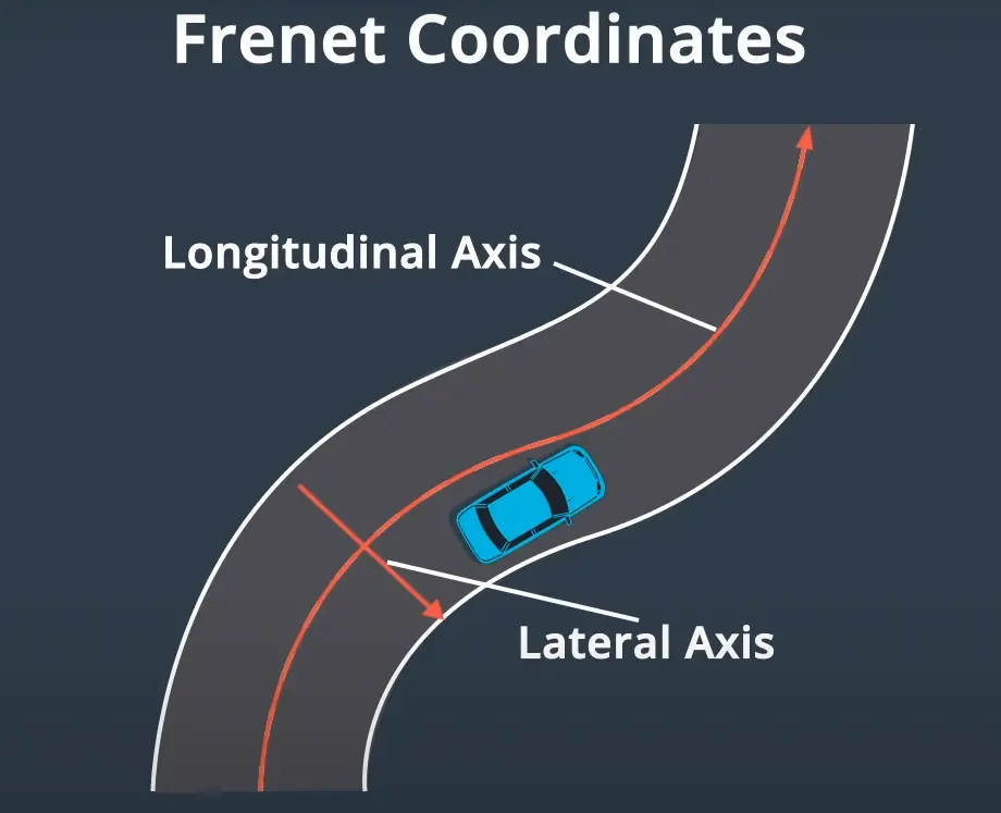
The Frenet frame takes the track’s reference line (centerline / racing line) as a new “straightened axis.” Imagine cutting the winding track and stretching it out into a straight ribbon.

• $s$ (longitudinal) — the distance traveled along the reference line from the start. “How far along the track have I gone?”
• $d$ (lateral) — the perpendicular offset from the reference line. “How far to the side of the center line am I?” (usually left $+$, right $-$)

1.3 Why Frenet Is Great for Racing

Almost every question you ask in racing — “am I ahead of the opponent or behind?”, “should I hug the inside or the outside of this corner?”, “is there room to overtake?” — comes down to how far along the track (longitudinal) and how far off to the side (lateral). The Frenet frame $(s, d)$ takes exactly these two axes as its coordinates, so even on a curved track these judgments become simple arithmetic.

A car driving along the track has the simple pattern “$s$ increases at constant speed, $d$ stays roughly constant” in Frenet. In $(x, y)$, the same motion makes $v_x,\ v_y$ swing wildly every time the track bends, which is hard to work with. So from racing-line planning to predicting an opponent’s motion to deciding on an overtake — many modules of the racing stack become far simpler on the Frenet frame.

In the demo below, watch the same constant-speed motion decomposed in the two frames. On the left, Cartesian splits the velocity into $v_x \cdot v_y$, so the values keep changing as the track curves; on the right, Frenet splits it into $v_s \cdot v_d$, keeping $v_s$ constant and $v_d = 0$.

2. Frenet ↔ Cartesian Conversion

The two frames convert into each other. All you need is the position $(x_r, y_r)$ and the heading angle $\theta_r$ (tangent direction) at each point of the reference line.

2.1 Frenet → Cartesian: $(s, d) \rightarrow (x, y)$

Given Frenet coordinates, this finds the actual $(x, y)$ on the map.

1. Find the reference point — use the given $s$ to locate the point $P_{ref} = (x_r, y_r)$ on the reference line.
2. Compute the direction vectors — at $P_{ref}$, get the tangent vector $\vec{t}$ and the normal vector $\vec{n}$. With path heading $\theta_r$, the normal is the tangent rotated by $90^\circ$: $(-\sin\theta_r,\ \cos\theta_r)$.
3. Move laterally — from the reference point, move a distance $d$ along the normal to get the final coordinates.

\[x = x_r - d\,\sin\theta_r, \qquad y = y_r + d\,\cos\theta_r\]

2.2 Cartesian → Frenet: $(x, y) \rightarrow (s, d)$

Given the vehicle’s global coordinates $(x, y)$, this finds where on the reference line it is ($s$) and how far off it is ($d$). This is also called projection onto the reference line.

1. Find the closest point — among the points on the reference line, find $P_c = (x_c, y_c)$ nearest to the current position $(x, y)$ (by searching discretized path points or by optimization).
2. Compute $s$ — accumulate (integrate) the arc length from the start of the reference line up to $P_c$.
3. Compute $d$ — the Euclidean distance between $(x, y)$ and $P_c$ is the magnitude of $d$. The sign (left/right) comes from the cross product of the tangent vector and $(x - x_c,\ y - y_c)$, which tells which side of the path the vehicle is on.

\[d = \operatorname{sign}\!\big(\vec{t} \times (P - P_c)\big)\,\lVert P - P_c \rVert\]

3. Things to Watch Out For

When actually using Frenet conversions, be especially careful about these two points.

• Overlap on a closed track — if the track length is $20\,\text{m}$, then $s = 0$ and $s = 20$ mean the same spot. When working with $s$, take it modulo the total length $L$ ($s \bmod L$) so that ahead/behind comparisons don’t break near the start line.
• Jumps in $s$ — during Cartesian ↔ Frenet conversion, if the closest point suddenly changes — especially near the track’s seam or a sharp curve — the value of $s$ can jump. Where continuity matters, mitigate this by searching for the projection only in the neighborhood of the previous $s$.

Drag the point (the car) in the demo below. The moment it crosses to the other side of the thin wall, the corresponding point on the reference line found by naive global nearest jumps to the opposite lane (red line), making $s$ jump discontinuously.

Wrap-up

This post covered the Frenet frame $(s, d)$, which takes a curved track as a straightened axis, and the two-way conversion with Cartesian coordinates.

• $s$ is the distance traveled along the reference line; $d$ is the lateral offset from it.
• Frenet → Cartesian moves a distance $d$ along the normal from the reference point; Cartesian → Frenet is a projection onto the closest point.
• Because motion on a curved track becomes so simple in Frenet, everything from racing-line planning to opponent prediction to overtaking decisions gets simpler across the racing stack.

Placing perception results (e.g., 2D LiDAR Detection & Clustering) on top of this Frenet frame lets us handle the opponent with a simple model even on a curved track.