Detection — Feature Extraction: Summarizing a Cluster as a Rectangle
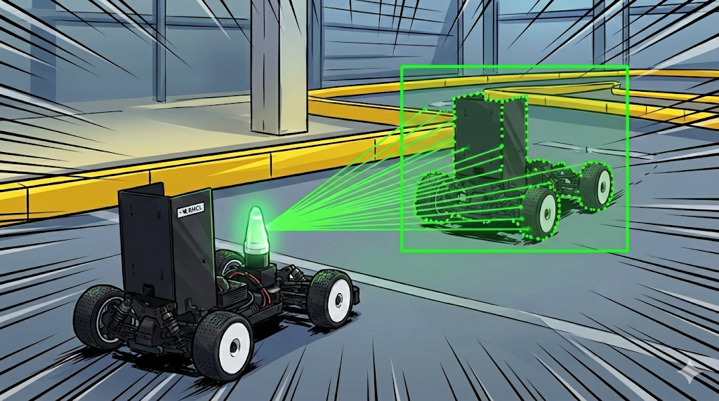
In the previous post, Detection & Clustering, we grouped scattered points into small pointsets via clustering. But a cluster is still just a “set of points.” Passing it to tracking as-is is a heavy representation, and you can’t know physical quantities such as the opponent’s orientation and size. So we need to extract a state (feature) that represents each cluster.
Rectangle Extraction
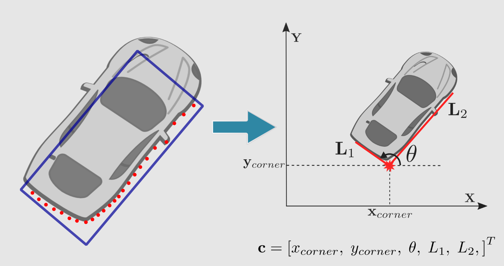
A car and its detection box are, in the end, close to a rectangle. So we summarize the opponent by finding a rectangle that encloses the cluster.
The method is simple. Sweep over all possible orientations $\theta$, build a rectangle enclosing the points at each orientation, and pick the orientation with the best score (highest or lowest, depending on the criterion). In the end you get a box summarizing the opponent as center · size · orientation ($\theta$).
The box obtained this way becomes a representation that lightly conveys not only the opponent’s position but also its heading and size to the tracking/prediction stages.
Two Criteria for Choosing the Orientation
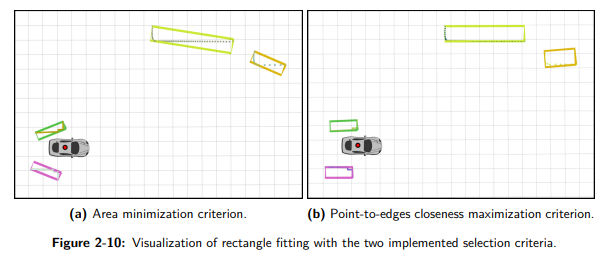
So, what do we use to judge the “best orientation”? There are two representative criteria — Closeness, which looks at how tightly points hug the edges, and Area Minimization, which looks at whether the enclosing area is smallest.
1. Closeness — the Orientation Where Points Hug the Edges
At each orientation, we project the points onto the rectangle’s two axes (edges) and score how tightly the points cling to an edge. When one edge aligns with the object’s real corner, the points concentrate on that edge and the score peaks.
In the demo below, the left animation shows the points being projected onto the x/y axes as the orientation $\theta$ rotates, and the right graph shows the closeness score at that moment. At $\theta^{*}$, where the score is maximal, you can see the edge fitting the corner exactly. Toggle between Full rectangle (all four edges visible) and Half (2 faces) (only two edges visible, as with a real LiDAR): closeness still peaks cleanly at $0°/90°$ even when only two faces are visible.
2. Area Minimization — the Orientation With the Smallest Enclosing Area
The other criterion picks the orientation where the rectangle’s (bounding box) area is minimal. The intuition is that the orientation enclosing the points most tightly is the object’s orientation.
But there’s a limitation. A real single-shot LiDAR only measures about two faces (an L-shape) of the object. When all four edges are observed, area minimization is accurate; but when only two faces are visible, the enclosing area becomes similar across many orientations, so the minimum point becomes ambiguous. In such cases the closeness criterion above is more stable.
In the demo below, compare how the bounding-box area changes with orientation, and how flat (ambiguous) the minimum becomes when only two faces are visible.
Wrap-up
We covered summarizing a clustered set of points by sweeping orientation $\theta$ into an enclosing rectangle, extracting center · size · orientation. For choosing the orientation there are the Closeness criterion (how tightly points hug the edges) and the Area Minimization criterion (the enclosing area); in a real LiDAR environment where only two faces (an L-shape) are visible, closeness is more robust.
The box (feature) extracted this way flows into the next stage, tracking/prediction, becoming the input for estimating the opponent car’s trajectory.