Track-ROI Filtering with Grid Filter
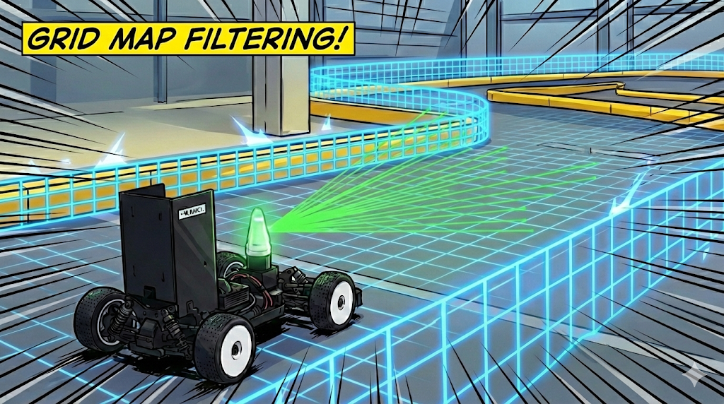
This post looks at Grid Filter — a utility that uses a static map (occupancy grid) to quickly answer “is this point inside the track (ROI)?”
Grid Filter really provides just one thing — is_point_inside(x, y): given a world coordinate, it answers True/False for whether it lies inside the drivable track. Two places consume this simple primitive.
- Detection ROI restriction — it limits LiDAR perception to the inside of the track. Points returned from outside the track (beyond a wall, etc.) are not added as clustering candidates. (→ Fewer walls mistaken for opponent cars; the reduced number of processed points is a side effect derived from here.)
- Path validity check — it checks whether a path the planner generated (spline / avoidance path) stays inside the drivable track.
In other words, the single function “use the map to tell inside/outside the track” supports both Detection and the Planner.
Core Idea
Before driving, we already have a static map of the track (an occupancy grid built with SLAM, etc.). White = drivable (track), black = wall / off-track.
The idea is two lines.
- Convert any world coordinate to a map pixel and read whether that spot is white or black — you instantly know “is it inside the track?”
- The area right next to a wall is ambiguous due to localization/map error, so shave the track region slightly inward from the walls (erosion) to leave a safety margin.
How It Works
1) Coordinate Conversion and Flip
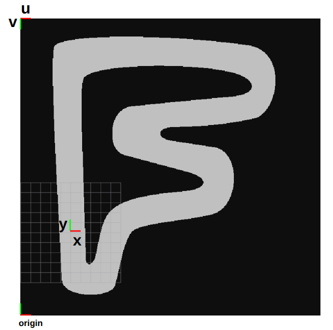
We map world coordinates $(x, y)$ to map pixels $(u, v)$.
\[u = \left\lfloor \frac{x - x_{origin}}{resolution} \right\rfloor, \qquad v = \left\lfloor \frac{y - y_{origin}}{resolution} \right\rfloor\]- $(x, y)$: world coordinates (unit: $m$)
- $(x_{origin}, y_{origin})$: world coordinates of the map
origin— by the ROS map convention, this corresponds to the bottom-left pixel of the image (unit: $m$) - $resolution$: physical size of one pixel (unit: $m/pixel$)
- $(u, v)$: pixel index ($Int$)
There is one thing to watch out for here. The $v$ formula above assumes “the row index grows upward (the origin row is at the bottom).” But depending on where you get the map from, the image’s row direction differs.
When loading from a PNG/PGM image file: an image file has row 0 at the top-left, so it is upside down relative to world $y$. Used as-is, lookups come out vertically flipped, so you must flip vertically once right after loading to put the origin at the bottom-left.
1
2
image = cv::imread(path, cv::IMREAD_GRAYSCALE);
cv::flip(image, image, 0);   // flipCode 0 = vertical flip (reverse rows)
When receiving an
OccupancyGridtopic: by the ROS convention,datais stored row-major starting from the bottom-left (0,0) (first +x, then +y). So afterreshape(H, W), row 0 is already at the bottom (origin), and you can index[v, u]directly without flipping. (If you display it withimshowit looks upside down, but that is only a display issue — the indexing math is correct.)
In short, flip exactly once, and flip yourself if the input is a PNG / not needed for an OccupancyGrid. (Flipping twice returns to the original, which is wrong.)
2) Making a Safety Margin with Erosion
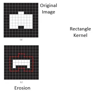
A point right next to the track boundary is ambiguous — wall or track? — because of position error. So we shave the drivable region (white) a little inward from the wall to leave a margin. OpenCV’s erosion does this — eroding the white (free) region effectively expands the black (wall) region by the same amount. (Erosion and dilation are a dual pair that swap when you invert foreground/background: erode(free) = dilate of the wall.)
An important point: the inward shave from kernel size $k$ is not $k$ but $(k-1)/2$ pixels. Since a rectangular kernel’s anchor is at the center, you retreat only by the “radius” from the wall.
\[d_{margin} = \frac{k - 1}{2} \times resolution\]| kernel_size | shave $(k{-}1)/2$ | physical margin ($res=0.05\,m$) |
|---|---|---|
| 1 | 0 px | 0.00 m (no erosion, max track width) |
| 5 | 2 px | 0.10 m |
| 11 | 5 px | 0.25 m |
e.g., at 5 cm resolution, kernel 11 → 5 px → a 0.25 m margin inward from the wall. (Kernel 5 is 0.10 m, not 0.25 m — be careful not to confuse kernel size with the actual shave width.)
3) Filtering Logic
The full pipeline is as follows.
- On map load (after flipping if needed), apply erosion once up front to build
eroded_image. (No per-frame recomputation.) - Convert an input point $(x, y)$ → pixel $(u, v)$.
- Look up
eroded_image[v, u]: 255 (white) → inside the track → True, 0 → outside → False. - In Detection, points that are False are excluded from clustering candidates immediately.
Because it looks up a precomputed image by coordinate, it is effectively a 2D lookup table (precompute-once, O(1) lookup).
Try adjusting the erosion kernel size in the demo below. The larger the kernel, the more the walls are inflated inward, and you can see right away how LiDAR points that fall inside that boundary get filtered out (grey = removed).
Parameters & Tuning
- Resolution — map resolution (e.g.,
0.05 m/px). Fixed by the map. - kernel_size — the only tuning knob. Margin = $(k{-}1)/2 \times res$.
- Small → maximum track width, keeping even points near the wall (risk of wall noise if localization wobbles).
- Large → generous clearance from the wall, suppressing false detection (but too large can erase real obstacles next to the wall).
- Kernel shape — currently rectangular (
cv::MORPH_RECT). Being rectangular, corners are shaved more along the diagonal (up to $\sqrt{2}\times$ the distance). If you want a uniform physical-distance (isotropic) margin from the wall, switch tocv::MORPH_ELLIPSE.
Results
Case 1 — kernel size 1
0 px erosion → secures maximum track width. However, wall noise can leak in during rapid movement.
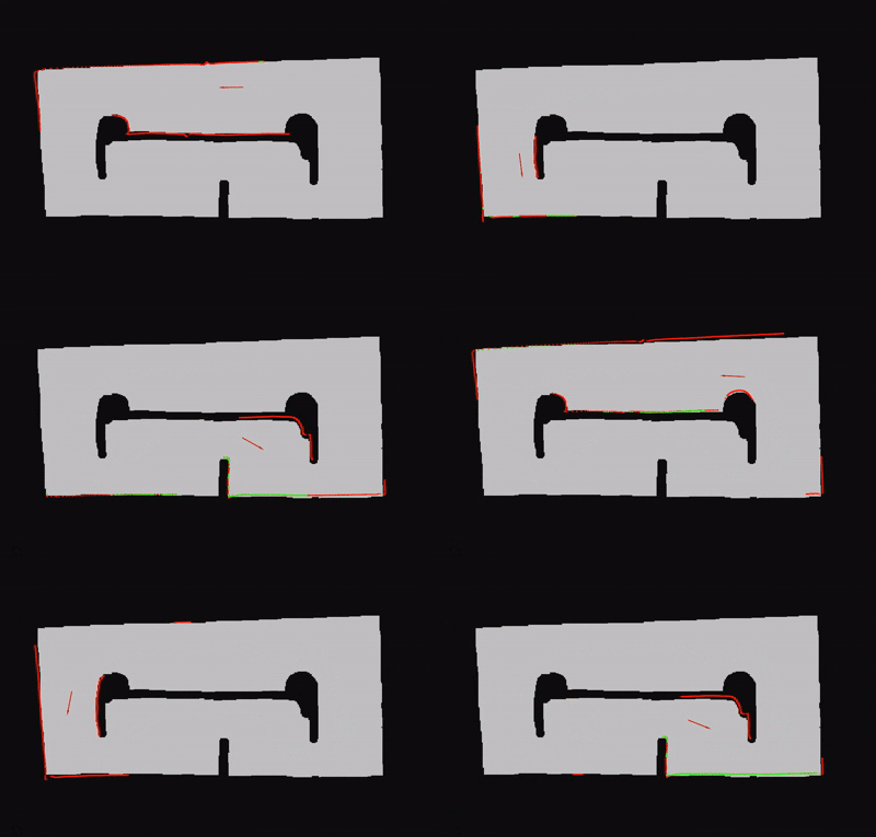
Case 2 — kernel size 11
5 px (0.25 m) erosion → secures ample clearance from the walls, giving excellent false-detection suppression.
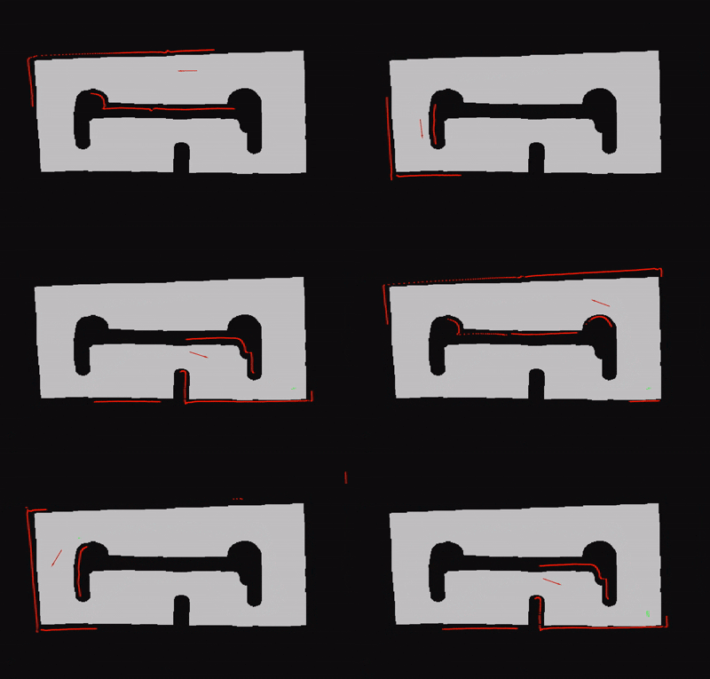
- Cluster generation restriction: points in the region where Grid Filter returns
false(the wall expanded by erosion) are excluded from the clustering input. - Conclusion: points entering the expanded wall region are ignored for cluster generation altogether, so perception reliability improves.
Assumptions & Limitations
Grid Filter only works properly under a few assumptions.
- It depends heavily on localization — you need to know where you are on the map (pose) to convert a point’s world coordinate to a map pixel accurately. The more accurate the localization, the more accurate the filter.
- It is vulnerable to rapid motion — if the pose wobbles, it can mistake a real obstacle inside the track for a wall and erase it. So robust localization is needed even under rapid motion; the kernel margin absorbs some of it, but too large a margin also erases real obstacles.
- It ignores map origin rotation (yaw) — the current implementation does not account for the
origin’s yaw, so if the map origin is rotated, the coordinate conversion needs extra handling. - It assumes a static map — the real track shape must match the map. Changes not in the map (a moved wall, etc.) are not reflected.
Wrap-up
Grid Filter is a simple but powerful utility that uses a static map to answer “is this point inside the track?” in O(1).
- One primitive, two consumers:
is_point_insidefor Detection ROI restriction + path validity check. - Coordinate conversion + flip: world → pixel conversion. Flip vertically once on load for a PNG; for an OccupancyGrid it’s already bottom-left row-major, so leave it as is.
- Erosion margin: shave the track $(k{-}1)/2$ pixels from the wall to secure a safety margin, tuned by the kernel.
- Less computation: excluding points on walls up front reduces the clustering load. Looking up a precomputed image, it’s effectively a LUT.
But all of this only holds if localization backs it up, so use it together with robust position estimation.