Opponent Trajectory Prediction with Gaussian Processes

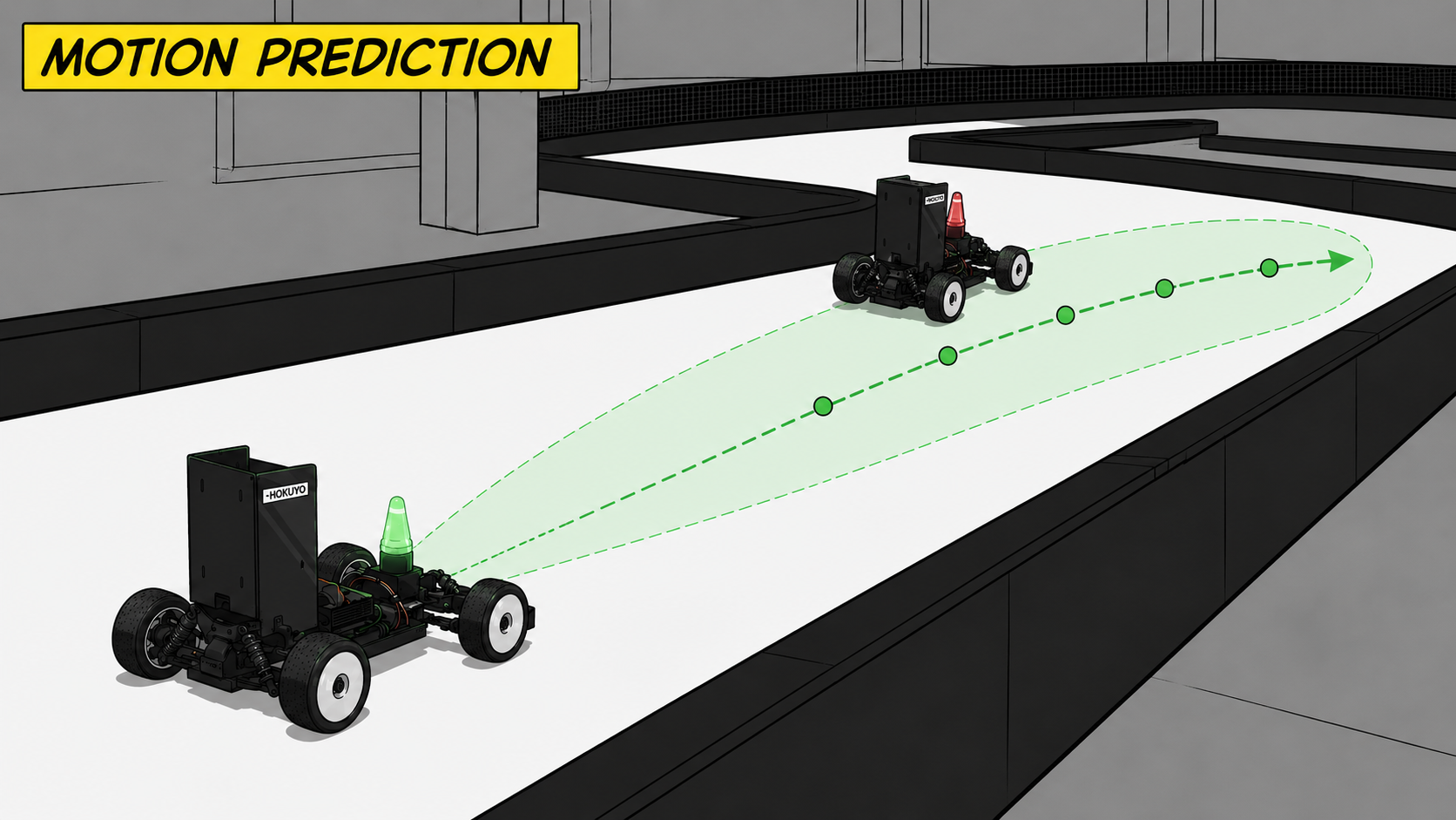
gp_traj_predictor learns the motion of the opponent detected by tracking to build the opponent’s driving line, and produces the future obstacle prediction that the planner uses. The key is handling the opponent’s position in Frenet coordinates ( $s$ = progress distance, $d$ = lateral deviation).

① Principle

After collecting opponent observations as $(s, d, v_s, v_d)$, Gaussian Process Regression estimates the line and speed as a function of $s$. The GP gives not only the mean but also the uncertainty (d_var, vs_var), partly visualized via RViz marker size/color.

\[d = f(s) + \epsilon\]

flowchart TD
    I["/tracking/obstacles<br>/car_state/odom_frenet<br>/global_waypoints"] --> A["opponent_trajectory.py<br>select opponent + Frenet observation history"]
    A -->|/proj_opponent_trajectory| B["gaussian_process_opp_traj.py<br>GP/CCMA interpolation → full trajectory"]
    B -->|/opponent_trajectory| C["opp_prediction.py<br>convert to future obstacle sequence"]
    C -->|/opponent_prediction/obstacles_pred| P["planner / state machine"]

File	Role
opponent_trajectory.py	select opponent from tracking + Frenet observation history
gaussian_process_opp_traj.py	interpolate observations with GP/CCMA into a full trajectory
predictor_opponent_trajectory.py	auxiliary return-trajectory prediction when the opponent leaves the line
opp_prediction.py	learned trajectory → future obstacle sequence for the planner

Key Steps

• Observation collection — from /tracking/obstacles, pick the closest opponent relative to ego and organize a Frenet $(s,d,v_s,v_d)$ history.

• GP trajectory generation — estimate $s\to d$ and $s\to v_s$ with a GP. Initially only the observed half-lap segment; once more than a lap accumulates, the whole lap. The discontinuity near the start line ( $s=0 \leftrightarrow s=L$ ) is handled with wrap-around by duplicating the leading/trailing segments.

• Return-to-line prediction — if an observation differs from the existing trajectory’s $d$ by more than 0.3 m, opp_is_on_trajectory=False → blend the latest detection with the existing line to generate a return trajectory (it does not assume infinite straight-line motion).

② Running It (RoboStack)

Prediction is launched as part of the full stack where perception (detect/tracking) and localization run together (perception package · opponent_predictor).

unicorn                    # conda env + CycloneDDS + workspace
cbuild
# full autonomy with a virtual opponent (prediction included)
ros2 launch stack_master headtohead.launch.xml sim:=true map:=f
# prediction alone: ros2 run perception opponent_predictor

• Inputs: /tracking/obstacles, /car_state/odom_frenet, /global_waypoints

• Outputs: /opponent_trajectory, /opponent_prediction/obstacles_pred, /opponent_prediction/force_trailing

Stack position: perception → tracking → prediction → planning → state machine → control

③ Results

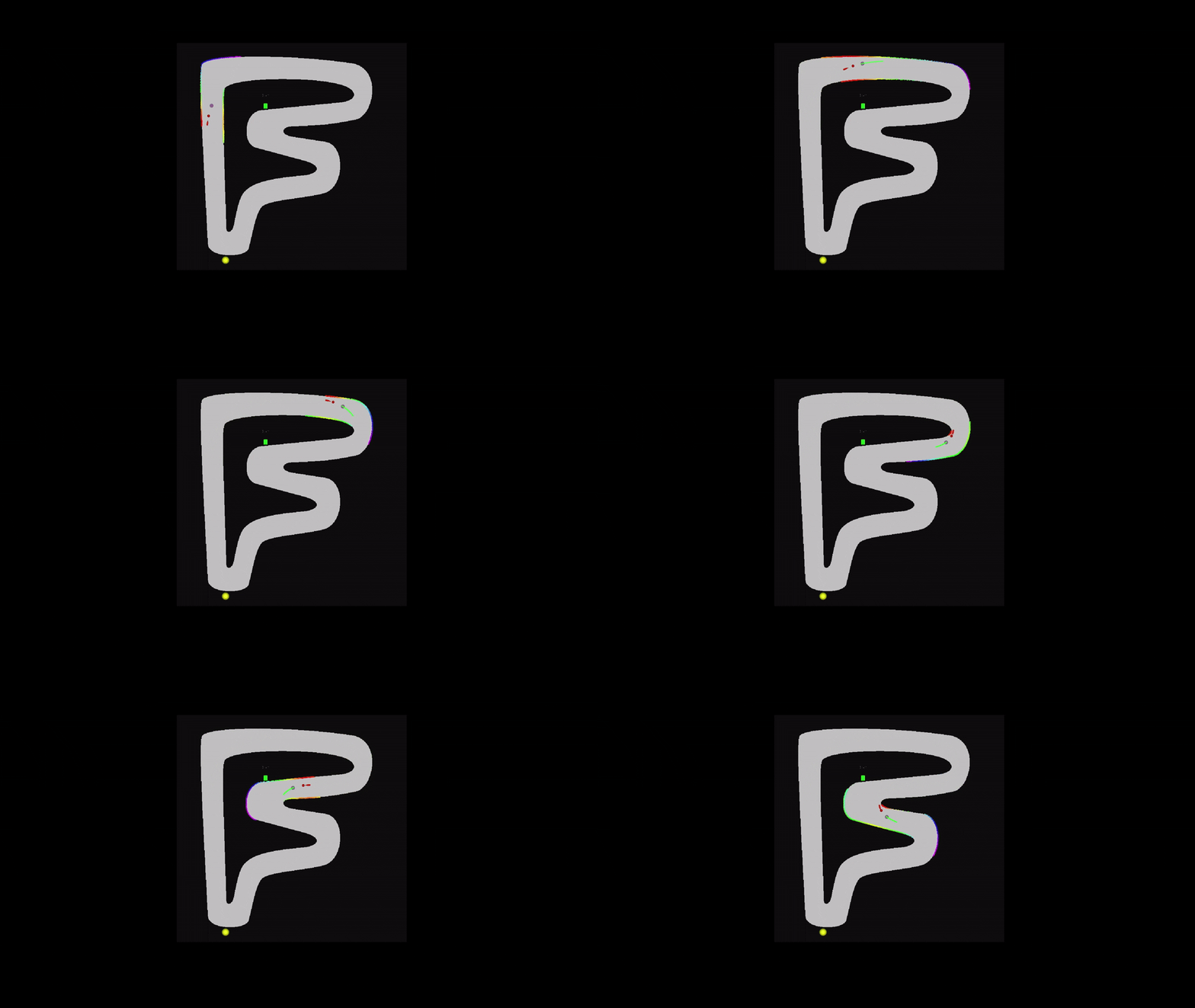
Half-lap observation stage — only the observed segment is updated by the GP:

Whole-lap trajectory — once more than a lap of observations accumulates, the opponent’s repeated driving line is generated:

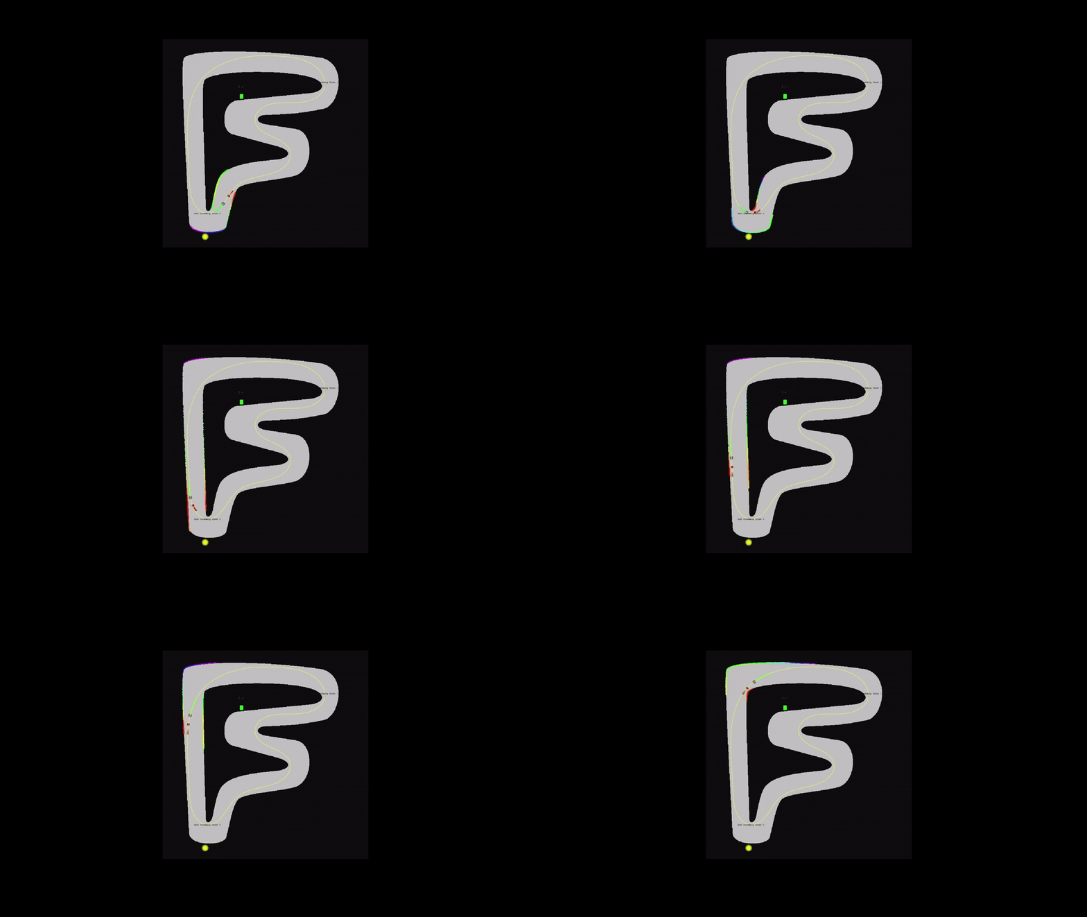
The mean + uncertainty from the GP becomes the basis for the planner’s avoidance/overtaking decisions.

Wrap-up

gp_traj_predictor interpolates the opponent observations from tracking in Frenet coordinates with a Gaussian Process, estimating the opponent’s repeated driving line and its uncertainty, and produces the future obstacle sequence the planner uses.

• Observation collection (Frenet) → GP estimates of $s\to d$, $s\to v_s$ → future obstacle prediction
• Provides not just the mean but also the uncertainty, informing avoidance/overtaking decisions

The /global_waypoints the GP uses as its reference frame is generated by Global Trajectory Optimization.